An Empirical Analysis of Continuous Poisson Distribution and Deep Learning Models in the Context of Financial Performance in Europe

Introduction

In the dynamic landscape of modern finance, understanding and managing financial risk has become a cornerstone of economic stability and institutional resilience. Financial risk refers to the possibility of losing money on investments or business operations due to market fluctuations, credit events, or macroeconomic factors. In this decade, financial services are main pillars to keep up the economic growth and stability of any country. Financial services play crucial role in fast-paced economy. Global economy is referred to the interconnected world. It is easier to understand the role of financial markets and institutions how much affecting the economy with the help of advance technology. One of the most critical aspects of financial risk management is the measurement and assessment of credit risk, particularly in the context of loan defaults. Loan defaults arise from where borrowers fail to meet their repayment obligations which leads to a significant threat to financial institutions, often signalling underlying economic distress.

This paper explores the complex interrelationship between financial risk and key economic indicators, focusing on how loan default rates, unemployment trends, and inflation dynamics can be used to enhance financial risk measurement frameworks in European economy. According to Aslam et al. (2019), loan lending has become a crucial component of global finance for many years [1]. If this continues, credit scoring serves as a vital tool for managing and accessing credit risk. The occurrence of loan defaults in Europe is closely intertwined with broader economic indicators, notably the unemployment rate and the inflation rate. Rising unemployment can lead to reduced consumer income, thereby increasing the likelihood of defaults on personal and business loans. Similarly, high inflation erodes purchasing power and can disrupt cash flows, making it more difficult for borrowers to service their debts. Hence, integrating macroeconomic variables like unemployment and inflation rate into financial risk measurement models is essential for more accurate forecasting and proactive risk mitigation.

The inflation rate represents the state at which the general level of prices for goods and services rises over time, leading to a decrease in the purchasing power. Inflation is typically measured through indices like the Consumer Price Index, CPI, and it plays a critical role in shaping monetary policy, consumer behaviour, and financial planning across all levels of the economy. There is a direct association between inflation rate and loan defaults, this means if inflation rate rise then loan defaults will also rise and vice versa. This happens because individuals and businesses may struggle to keep up with rising costs while their incomes or revenues remain stagnant. In response to inflation, apex banks often raise interest rates, which can increase loan repayment amounts for borrowers with variable-rate loans. The combined pressure of higher living costs and increased debt servicing requirements can make it difficult for borrowers to meet their obligations, ultimately leading to a higher risk of loan default.

The unemployment rate measures the percentage of the labour force that is actively seeking but unable to find work. High unemployment often signals economic weakness, as businesses reduce hiring or lay off workers due to declining demand, financial constraints, or broader market uncertainty. When unemployment rises, it affects household income levels and reduces overall consumer spending, which can further dampen economic growth. A high unemployment rate can lead to an increase in loan defaults and can also have complex effects on inflation. At the same time, high unemployment typically reduces consumer demand, which can put downward pressure on prices and slow inflation. Regardless of the inflationary impact, the connection between unemployment and loan default remains strong, as loss of income is one of the primary drivers of financial distress among borrowers.

Literature Review

According to JPK Gross et al., 2009, the effects of financial aid policies have been studied with difficulty due to their volatility but some areas like student debt, the issue of student loan defaults has not been thoroughly examined using large national datasets for over a decade [2]. According to Lin Zhu et al., 2019, predicting loan default can be built by using deep learning algorithm, and the results are compared with statistical models [3]. According to Barbaglia et al., 2023, loan defaulters are considered as crucial for policymakers to reduce costs and prevent inefficient resource allocation [4]. If the past dataset, which contains information on millions of residential mortgages and borrowers across many countries, is studied, with default occurrence predicted by using various statistical techniques, machine learning, and deep learning models.

According to Hur et al., 2018, inflation cyclicality impacts borrowing costs, debt dynamics, and defaults [5]. Therefore, observing inflation rate estimates the co-movement between inflation and consumption growth fluctuates across advanced countries, with stronger co-movement linked to lower borrowing costs in stable periods. Hence, inflation cyclicality helps explain interest rates and default dynamics. In the benchmark model, economies with procyclical inflation face lower borrowing costs but higher default risks during downturns. As inflation falls, the real debt burden rises, increasing the likelihood of a debt crisis and magnifying countercyclical default risks.

According to Guadencio et al., 2019, the preponderance of lending standards as default rate drivers is quantified with a unique dataset providing insights for supervisors in the selected area [6]. Loan defaults are intended to guide policy decisions regarding bank lending practices across euro area countries. According to Bai, 2021, labour market moments are present as the growing economy for any country [7]. Benchmark and all-equity models, are used to report unemployment volatility and skewness across simulations. The analysis used to present a strong relationship between credit spreads and unemployment, with labour market conditions significantly impacting credit risk. According to Niu et al., 2015, job losses are directly affected on foreclosure is concluded using data from any region or any country and a job loss is a vulnerability index, which measures the spatial relationship between employment and residential locations [8]. The spatial separation between job and housing locations is shown to significantly affect foreclosure rates, supporting the double trigger theory. The study suggests that increasing unemployment benefits could mitigate job loss impacts on foreclosures, promoting housing market stability.

According to Quercia et al., 2016, the impact of borrower unemployment as a trigger event for mortgage default using than lower income earning citizens and minority borrowers [9]. Unemployment is found to be a significant predictor of default, complementing the traditional unemployment rate. Both household unemployment and equity position are shown to influence default decisions, supporting the trigger event and option-based views. Increase in unemployment rate may offer more precise predictions of mortgage default and calls for further research on underemployment and unemployment benefits. According to Hurtin et al., 2018, estimating loss function is essential for financial risk analysis with inflation rate as it quantifies the deviation between predicted and actual outcomes, guiding model optimization [10]. Loss function helps assess the impact of inflation on investment portfolios and credit risk by evaluating inflation rate. This leads to accurate risk prediction and strategy formulation in inflation- sensitive financial environments.

According to Chen 2022, evaluation of loss function is essential to do the financial risk analysis with unemployment rate as it helps measure the discrepancy between predicted and observed outcomes, optimizing model performance [11]. Integrating the unemployment rate with the loss function allows for a more accurate assessment of its impact on loan defaults, credit risk, and market instability. According to Yang et al., 2016, gamma function is necessary in financial risk analysis because it helps model distributions of financial variables that are skewed or heavy-tailed, which are common in risk assessments. Gamma function used in risk metrics like Value at Risk (VaR). According to Marsaglia et al., 1986, continuous Poisson distribution is known as incomplete gamma function [12]. Continuous Poisson distribution, is essential to estimate risk and analysing the risk. This distribution only works for asymmetric data types. Risk is also asymmetric because both tail can not be measured equally, therefore CPD leads to better understanding the model and the volatility of the past data.

According to Mashur et al., 2020, Machine learning models have a pivotal role in financial risk analysis by enabling the identification of complex patterns in vast datasets [13]. ML models adapt historical data and making them valuable tools for dynamic financial environments, allowing various methods to better manage and mitigate risks in an increasingly complex market landscape. According to Stevenson et al., 2021, deep learning models are essential for financial risk analysis as they can process large amounts of data and identify complex patterns [14]. DL models improve predictive accuracy in assessing credit risk, market fluctuations, and potential loan defaults. Their ability to learn from historical data allows for more informed decisionmaking and better risk management strategies.

Methodology

Financial risk measurement is essential for observing the development of economic growth because it ensures financial stability, boosts investor confidence, and supports informed decision-making. If potential threats like loan defaults, market volatility, or liquidity issues, can identified then businesses and governments can take early action to minimize losses and avoid economic disruptions. When the distribution of data is not balanced or evenly spread is known as asymmetric data, which means one class or group has significantly more samples than others, leading to class imbalance. In this study, loan default data is also asymmetric because the number of people who repay loans is usually much higher than those who fails to repay loans. This creates a class imbalance, in the dataset. Loan defaults are relatively rare, the dataset becomes skewed, making it harder for models to learn and accurately predict the cases.

A well-managed financial system encourages investment. If market risks are predictively analysed and controlled, investors are more likely to fund businesses, fuelling innovation, job creation, and overall productivity. This flow of capital is essential for a growing economy. Therefore, Exploratory Data Analysis, EDA is a crucial first step before analysing financial risk because it helps to understand the underlying patterns, detect anomalies, and prepare data for more complex modelling. Without a clear understanding of this data, risk assessments can be misleading or incomplete. EDA provides insights into data distribution, trends, and relationships between variables. In financial risk analysis, a loss function analyses the cost associated with prediction errors. It is crucial for building models that assess or forecast risk, as it guides optimized models are trained to minimize this function. Basically, loss function reflects the trade-off between false positives and false negatives, making it essential for accurate and practical risk management.

The Laplace distribution is used in financial modelling because when modelling error terms or returns where sharp spikes are likely. The heavier tails of Laplace distribution provide more realistic risk estimates, especially for value-at-risk, VaR or stress testing. This helps in preparing for rare but severe events, improving financial resilience. The Pareto distribution is vital in modelling extreme financial risks, especially in the tails of the loss distribution. Pareto distribution follows the 80:20 rule, often applicable in finance where a small percentage of events cause a majority of losses. To measure the risk measurement, Pareto allows institutions to understand and hedge against rare, high-impact events, which traditional models might underestimate.

Monte Carlo simulations are computational algorithms that rely on repeated random sampling to obtain numerical results. Specially, it is used to examine numerous trials using random inputs drawn from probability distributions to simulate a complex process or system. In this technique, Value at Risk (VaR) is used to measure the potential loss in value of an asset or portfolio over a defined period for a given confidence level. VaR estimates the maximum loss that is not expected to be exceeded with a specified probability. Continuous Poisson Distribution, CPD or the incomplete gamma function is important in financial risk analysis because it appears in the mathematical modelling of distributions used to describe rare events, extreme losses, and time-to-event data—key areas in risk management. The incomplete gamma function is used to compute cumulative probabilities for distributions like the gamma and chi- squared distributions, which model the time until an event occurs. This allows analysts to estimate the likelihood of default over a specific period, which is critical for pricing loans, setting interest rates, or managing portfolio risk. Therefore, in loss modelling, especially under compound loss models, the continuous Poisson distribution helps to evaluate tail probabilities to assess the chance of large aggregate losses.

Deep learning models is crucial to analyse in financial risk to excel at modelling sequential and time-dependent data, like stock prices, credit scores, or transaction patterns. Traditional deep learning models often detect subtle signals in financial time series, forecast market volatility, or predict the likelihood of credit defaults based on historical behaviour. They also adapt well to nonlinear, high- dimensional data, making them powerful tools for identifying emerging risks that simpler models may miss. Overall, deep learning networks enhance prediction accuracy and provide a dynamic, data-driven approach to managing financial risk in real time.

Analysis

The dataset has been collected from European Central Bank website. Data has been collected from 31-01-2004 to 28-02-2025. There are total number of 254 entries. It is a monthly based dataset on loan defaults, inflation rate and unemployment rate. Descriptive statistics has been provided below to better understanding of the dataset.

                                                                               Table 1: Descriptive Statistics
The average adjusted loan value in the European data is 3.39, with a moderate degree of variability of 2.93. Inflation shows a mean of 2.13 and a standard deviation of 1.98, suggesting inflation rates fluctuate considerably. Finally, the unemployment rate averages 9.00 with a lower standard deviation of 1.72.

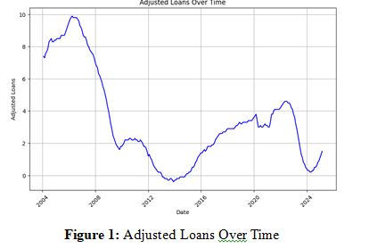
The adjusted loan values in Europe show considerable volatility over the period from 2004 to 2024. It is cleared that there was a sharp decline following the 2008 financial crisis, reaching a low around 2012-2014. A subsequent gradual increase occurred until around 2020, followed by another downturn and a recent slight uptrend at the end of 2024.

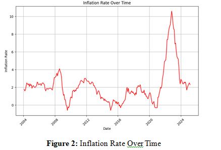
European inflation rates have fluctuated significantly between 2004 and 2024.In Figure-2 it is observed that, inflation in Europe saw peaks around 2008 and again very sharply around 20222023.

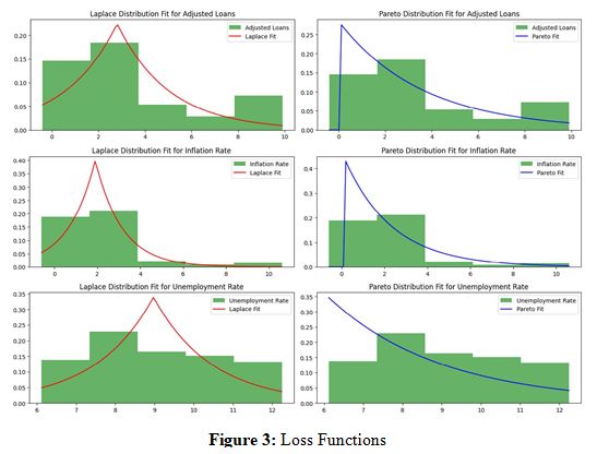
Figure-3 displays histograms of adjusted loans, inflation rates, and unemployment rates in Europe, overlaid with fitted Laplace distributions and Pareto distributions. For adjusted loans and inflation, both distributions show some divergence from the empirical data, particularly at the extremes. It is also shown that the distribution function of unemployment rate appears somewhat better approximated by both the fitted Laplace and Pareto curves.

                                                                         Table 2: Monte-Carlo Simulations
The Monte Carlo simulations yielded mean values of 2.77 for adjusted loans, 1.90 for the inflation rate, and 9.00 for the unemployment rate in Europe. When these three variables were combined, the simulation produced a mean of 13.67. These simulated means provide an estimate of the expected central tendency for each individual variable and their sum based on the underlying probabilistic models used in the simulation.

                                                       Table 3: Value-at-Risk at 95% Level of Significance
At a 95% confidence level, the VaR for adjusted loans is -2.48, suggesting that there is a 5% chance of losses exceeding 2.48 units. For inflation, the VaR is -1.01, indicating a 5% probability of inflation decreasing by more than 1.01 percentage points. The VaR for unemployment rate is 5.58, implying a 5% chance of the unemployment rate increasing by more than 5.58 percentage points.

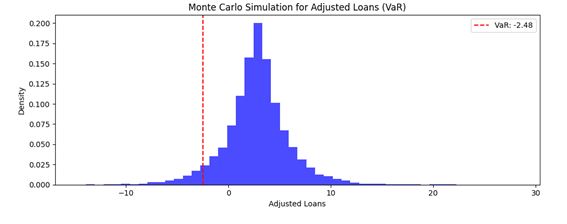
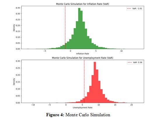
Figure-4 presents the simulated probability distributions for adjusted loans, inflation rates, and unemployment rates in Europe, generated through Monte Carlo simulations. It is observed that the unemployment rate simulation shows a distribution skewed towards higher values, suggesting a greater likelihood of unemployment rates exceeding the central tendency in the simulated scenarios. The above figure also displays the results of Monte Carlo simulations, with vertical dashed red lines indicating their respective Value at Risk at a 95% confidence level. It can be observed in Figure-5 that the VaR lines are positioned on theleft side of the distribution, marking the threshold below which 5% of the simulated outcomes are expected to fall. Now, to check the linearity between the variables, Ordinary Least Square, OLS method has been applied. To examine the effect of loan defaults with the volatility of inflation rate and unemployment rate OLS method is used. Therefore, loan default is taken as dependent variable and inflation rate and unemployment rate both the variable taken as independent variables to observe the time-to- time variation in Europe.

                                                                                   Table 4: Ordinary Least Square 

From the above Table-5, it is examined that low R-squared value is 0.138, which indicates that only about 13.8% of the variation in adjusted loans is explained by two independent variables inflation rate and unemployment rate. The statistically significant F-statistic value 8.65E-09 (< 0.001) suggests that the model as a whole is better than a null model with no predictors. It is also examined that coefficient for unemployment rate value of -0.6013 (<0.001) is statistically significant, implying that higher unemployment is associated with a decrease in adjusted loans. However, the coefficient for inflation rate value of 0.0454 is not statistically significant as p = 0.650, suggesting that inflation rate does not have a significant linear relationship with adjusted loans in this model.

Here, Durbin-Watson statistic of 0.003 indicates strong positive autocorrelation in the residuals, which violates a key assumption of OLS regression and suggests the model might be mis specified or the standard errors are unreliable. On the other side, the Jarque-Bera test strongly rejects the null hypothesis of normally distributed residuals (p < 0.001), further indicating potential issues with the model's assumptions.

                                   Table 5: Generalised Linear Regression Model with Continuous Poisson Distribution

Table-6 presents the Generalized Linear Model (GLM) by using CPD, where a log link function was used to model the dependent variable, suggesting an assumption that the variance of adjusted loans is proportional to the square of its mean. This GLM-CPD model was fitted using Iteratively Reweighted Least Squares, IRLS with 253 observations. However, the Loglikelihood and Pseudo R2 (CS) values cannot be calculated, which indicates a problem during the model fitting process or in the calculation of these statistics. The deviance is 1723.2, and the Pearson â?»2 is 251 with 250 degrees of freedom for residuals.

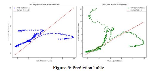
Figure-4 displays scatter plots comparing the actual adjusted loan values against the predicted values from OLS and GLM-CPD. In both models, the red line represents a perfect fitted curve where predicted values matched with actual values. In Figure-4, OLS model shows a cluster of predictions which does not closely align with the perfect fit line, particularly for higher actual adjusted loan values, which indicates a poor predictive performance. But, on the other hand GLM-CPD model predictions are following the trend of the actual values more closely than OLS model, especially in the lower to middle range. GLM-CPD is also shows some deviation from the perfect fit line, particularly at higher actual values, indicating that while potentially better than OLS.

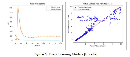
Figure-6 contains two plots Loss Over Epochs, and Actual vs Predicted Adjusted Loans. Here, the plot showing Loss over Epochs, examines the training loss and validation loss over 200 epochs. The training loss decreases rapidly in the initial epochs and then plateaus at a low value, which indicates the model learns well on the training data. But the validation loss initially decreases, then spikes dramatically before gradually decreasing and stabilizing at a higher level than the training loss. This pattern suggests overfitting, where the model starts to perform worse on unseen data after a certain number of epochs. But the other plot showing Actual vs Predicted Adjusted Loans, displays the relationship between the actual adjusted loan values and the predicted values from the model. The red line represents a perfect prediction. The predictions seem to be clustered in a narrow range, to reinforces the issue of overfitting observed in the loss plot, where good performance on training data doesn't translate to accurate predictions on unseen data.

Conclusion

In this study, the analysis of European loan defaults with respect to inflation rates, and unemployment rates reveals that these economic variables exhibit complex behaviour over the period from 2004 to 2024. Adjusted loan values and inflation rates are shown to experience considerable volatility, with significant fluctuations observed around key economic events. While the unemployment rate demonstrates less variability, exhibiting in a notable range. Loss distributions of these variables are not well-approximated by either the Laplace or Pareto distributions. Furthermore, the predictive performance of different models is evaluated. To ensure that GLM-CPD is found to be a more suitable choice for predicting adjusted loans compared to OLS regression. This conclusion is supported by a visual comparison of actual versus predicted values, where the GLM-CPD demonstrates a closer alignment with the observed data.

The task of predicting economic variables such as loan defaults inherently involves the selection of appropriate statistical distributions and robust analytical techniques. Throughout this analysis, different statistical modelling approaches were applied to gain insights into the dynamics of financial risk. Therefore, a more exploration of the CPD, should be undertaken to fully ascertain its predictive power and reliability for these European economic indicators. There are more statistical techniques, machine learning algorithms and deep learning algorithms and reinforcement learning algorithms can be used with CPD contexts to solve the future the financial risks. It analysed better than loss distributions and OLS. Each and every financial datasets are asymmetric, hence exploration with CPD will be a better choice. Better economic condition makes a country and a continent better [15-19].

Further Scope of the Research
In this era, technology is evolving day by day. New machine learning algorithms are coming to analyse the market volatility. New methods of deep learning and reinforcement learning are also inventing and innovating to develop the economy of any nation. In future there will be more advanced statistical tools, algorithms
available to get perfect prediction. Also CPD will be used to develop deep learning models to have perfect predictions and remove the obstacles in growing economy.

Limitations of this Research
Research on financial risk may face inherent uncertainty of predicting future. Assuming variables can be fluctuating every time and may not follow the loss distributions or gamma functions. Furthermore, the complexity in the global economy vary with different times with respect to growing technology and other variables such as nature volatility.

Ethical Standards
The research work was conducted in adherence to the highest ethical standards, with integrity and transparency. In this paper, all findings and analyses were presented with honesty and without bias or manipulation.

Funding
Author did not get any funds for this research.

Declaration of Interest
Author has no conflict of interest.

Data Sharing Statement
Data is available on ECB data website.

References

1.    Aslam, U., Tariq Aziz, H. I., Sohail, A., & Batcha, N. K. (2019). An empirical study on loan default prediction models. Journal of Computational and Theoretical Nanoscience, 16(8), 3483-3488.

2.    Gross, J. P., Cekic, O., Hossler, D., & Hillman, N. (2009). What Matters in Student Loan Default: A Review of the Research Literature. Journal of Student Financial Aid, 39(1), 19-29.

3.    Zhu, L., Qiu, D., Ergu, D., Ying, C., & Liu, K. (2019). A study on predicting loan default based on the random forest algorithm. Procedia Computer Science, 162, 503-513.

4.    Barbaglia, L., Manzan, S., & Tosetti, E. (2023). Forecasting loan default in Europe with machine learning. Journal of Financial Econometrics, 21(2), 569-596.

5.    Hur, S., Kondo, I., & Perri, F. (2018). Inflation, Debt, and Default.

6.    Gaudêncio, J., Mazany, A., & Schwarz, C. (2019). The impact of lending standards on default rates of residential real estate loans (No. 220). ECB Occasional Paper.

7.    Bai, H. (2021). Unemployment and credit risk. Journal of Financial Economics, 142(1), 127-145.

8.    Niu, Y., & Ding, C. (2015). Unemployment matters: Improved measures of labor market distress in mortgage default analysis. Regional Science and Urban Economics, 52, 27-38.

9.    Quercia, R. G., Pennington-Cross, A., & Tian, C. Y. (2016). Differential impacts of structural and cyclical unemployment on mortgage default and prepayment. The Journal of Real Estate Finance and Economics, 53, 346-367. 

10.    Hurlin, C., Leymarie, J., & Patin, A. (2018). Loss functions for loss given default model comparison. European Journal of Operational Research, 268(1), 348-360.

11.    Chen, H. (2022). Prediction and analysis of financial default loan behavior based on machine learning model. Computational Intelligence and Neuroscience, 2022(1), 7907210.

12.    Marsaglia, G. (1986). The incomplete Γ function as a continuous Poisson distribution. Computers & Mathematics with Applications, 12(5-6), 1187-1190.

13.    Mashrur, A., Luo, W., Zaidi, N. A., & Robles-Kelly, A. (2020). Machine learning for financial risk management: a survey. Ieee Access, 8, 203203-203223.

14.    Stevenson, M., Mues, C., & Bravo, C. (2021). The value of text for small business default prediction: A deep learning approach. European Journal of Operational Research, 295(2), 758-771. 

15.    Abid, S. H., & Mohammed, S. H. (2016). On the continuous poisson distribution. Int. J. Data Envelopment Anal. Oper. Res, 2(1), 7-15.

16.    Bening, V., & Korolev, V. (2022). Comparing compound Poisson distributions by deficiency: continuous-time case. Mathematics, 10(24), 4712.

17.    Jumaa, M., Saqib, M., & Attar, A. (2023). Improving Credit Risk Assessment through Deep Learning-based Consumer Loan Default Prediction Model. International Journal of Finance & Banking Studies, 12(1).

18.    Tanoue, Y., Kawada, A., & Yamashita, S. (2017). Forecasting loss given default of bank loans with multi-stage model. International Journal of Forecasting, 33(2), 513-522.

19.    Xia, S., Zhu, Y., Zheng, S., Lu, T., & Xiong, K. (2024). A Deep Learning-based Model for P2P Microloan Default Risk Prediction. Spectrum of Research, 4(2).