Wi-SUN FAN Network Re-formation Characterization

Index Terms

Wi-SUN FAN, Re-Formation, Timing, Mesh Network

Introduction

In a recent demonstration to the Wi-SUN Alliance membership Exegin Technologies Limited used its network simulation software to provide a realistic real time demonstration of WiSUN FAN network re-formation [1].

Network re-formation occurs when an entire network returns to operation after having suffered from a power loss such that all of the nodes in the network restart. A typical case where this may occur is when a portion of the power grid becomes de-energized, leaving many homes and businesses without power and hence the associated electricity meters as well. And subsequently the power is restored with the electric meters re-starting and resuming communications . Another is in a street lighting scenario where the power to the lights and the controlling electronics is turned off at day break and restored at dusk.

That this is network re-formation and not simply network formation is that it is assumed that each of the nodes has been authenticated onto the network, previously, and has retained its security material over the course of the power failure. Under these conditions the nodes can skip the authentication stages of joining a network. Network formation, consequently, will take longer, but that scenario was not part of this study. The underlying simulation software functions at the physical layer providing accurate modelling of the interaction of radio frequency nodes in a metrically correct deployment. The software, in this case, uses a free space path-loss model, which in comparison with physically comparable deployments has been shown to be similar in behaviour across a broad range of metrics; thereby representing a digital twin for actual deployments.

The layout of the nodes in the test FAN is shown in Figure 1, with Wi-SUN FAN border router at the centre of the grid.

Figure 1: 530 Node FAN Layout

As the name of the overall technology, ”Low Power Lossy Networking” foretells, in the underlying nature of the radio communication, that there is a degree of randomness in the behaviour of these network. Randomness that, in this case, is manifest in the distributions of the network re-formation times. 1

Disclaimer

We note that the results portrayed here are for a fully compliant Wi- SUN FAN 1.0 implementation. However, it is an implementation from Exegin Technologies, only, and for an ideal free space environment. As such, the behaviour to be obtained from other implementations or functioning in other, less ideal, environments may be different.

Wi-SUN FAN Network Re-Formation Simulation

For the first simulation we choose a set of 530 Wi-SUN FAN nodes (23 by 23 nodes plus a border router) that were positioned on a perturbed rectangular grid with an average inter-node spacing of 1000 meters as a representative network topology. Other configurations can also be simulated, from stars to string of pearls, dense or sparse, or combinations thereof but were not reviewed for this paper.

Each node in this system is a Linux process that executes an independent implementation of Exegin’s Wi-SUN FAN protocol stack and commensurate IEEE 802.15.4 MAC layer along with a thin application/node management component on top of the stack [2].

The nodes were calibrated to have a transmit power of 0 dBm and a receive sensitivity of -100 dBm.

The system was set to use the North American sub-GHz band of 902-928 MHz, FSK with a symbol rate of 300 ksym/s and to use 16 channels for the channel hopping plan.

A free space path loss model was used resulting in a pathloss of ∼91.7 dB per kilometre using an antenna of 0 dBm gain. 

The average density i.e. the average number of nodes in the network that any node might be able to receive transmissions from is ∼16.6 nodes/node.

Gaussian noise with a signal to noise ratio of 75 dB (worst case) was introduced to provide random interference.

Typical Network Re-Formation

The simulation was allowed to run, many times, and demonstrated a typical evolution that is shown in the follow set of figures. Each figure capturing the FAN’s join state at different instances in time as the network re-forms, starting at the one minute after the system was started.

Figure 2: FAN State at t0 Plus 1 Minute

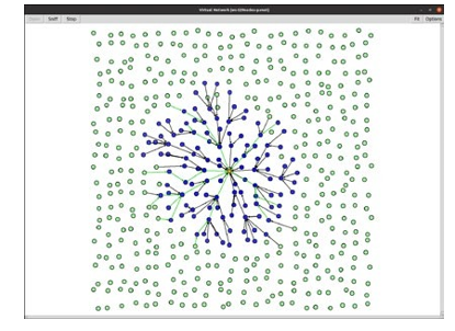
Figure 3: FAN State at t0 Plus 2 Minutes

Figure 4: FAN State at t0 Plus 3 Minutes

Figure 5: FAN State at t0 Plus 7 Minutes The Progress of the Re-Formation in Terms of the Evolution of the Number of Nodes Joined in Time is Shown Below in Figure 6.

Figure 6: Re-Formation Progress

The statistics for this run are:

Total Nodes: 529

Joined Nodes: 529

Join Rate: 1.34/s (1 node every 0.75 sec)

Duration: 6 min 36 sec

The system displayed the expected behaviour of initial exponential growth followed by saturation once the number of nodes remaining to join diminishes. The time to reach specific percentages of completion for this run are detailed in Table I.

                                                                   Table 1: Typical Re-formation Progression Percentages

Network Density

The behaviour of a mesh is critically dependant on the density of nodes in the network as defined by the average number of nodes that any one node might receive packets from, on the basis of whether the transmitted power of a packet from a node at the receiver is above or below its receive sensitivity. For this network, Figure 7 shows the density as experienced by each node in the network.

Figure 7: Network Density

The average density for this network is ∼16.6 nodes/node.

Other Sized Networks

In addition to the 530 node network we also analyzed networks of other sizes; 100, 256, 1024 in order to garner a broader set of statistical data regarding network re-formation. All of the properties of the networks remained the same inclusive of node spacing, radio characteristics and, hence, density, etc. except overall number of nodes and consequently network area.

Network Re-formation Statistics

Given the random nature of the neighbor selection process, especially given the channel hopping that each node is performing and as a consequence of Gaussian noise being introduced into the simulation, each simulation run of a network reforming exhibits different characteristics, one being the overall re-formation time for the entire network. The Figures 8 and 9 show the probability and the associated probability density of a network being re- formed in time t.

Figure 8: Network Formation Probability Curves (part1)

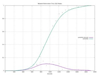
Figure 9: Network Formation Probability Curves

The averages and standard deviations for these distributions are detailed in table

         Table 2: Tabulated Average Re-Formation Time by Network Size and the Associated Standard Deviation

In addition we also provide the re-formation profile for the same set of networks. The figures in Figure 10 show the network re-formation process in terms of the numbers of nodes joined as a function of time.

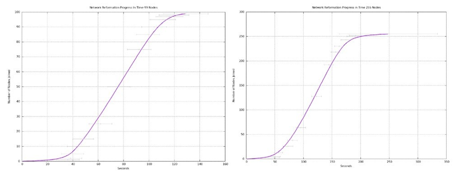
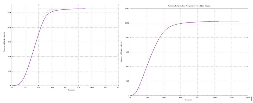
Figure 10: Network Formation Process Curves and Lastly, in Summary the Network Re-Formation Process Shown at States of 25%, 50%, 75%, 90%, 95% and 100% Complete

Conclusions

There is a direct correlation between the size of a network and the length of time that the network takes to reform as detailed in Table II and depicted in Figure 11.

Figure 11: Summary of Network Re-formation Process

The rate of re-formation follows the expected initial exponential growth followed by an exponential tail as the network re-formation approaches completion. In general the majority of the network, 90% is reformed in some 60% of the total time for the network to become completely re-formed i.e. the last %10 of the nodes take approximately 40% of the total elapsed time. In practical terms, e.g. for an electric meter deployment, the majority of the meters are reachable via the Wi-SUN FAN in a relatively short period of time.

That the rate of node re-joining tapers off as the network becomes more fully reconnected is also due, in part, to the trickle timers being used to moderate the behavior of a re-joining node: as time goes on from restart, the node will attempt to re-join the network less and less frequently. As such, the nodes that were furthest from the 6LBR on network restart; nodes that could not re-join immediately since there were no parent nodes to re-join, are waiting longer and longer to attempt to re-join [3].

The node discovery algorithm relies on the chance event of a node that has already re-joined the network receiving a beacon from a node that is attempting to re-join the network. Since the nodes are hopping on randomly selected channel plans the chances that a re-joined node will receive a beacon from a rejoining node is randomly distributed in time. A macro effect of this randomness at the node level is manifest in the statistically broad range of network re-formation times recorded.

References

1. IEEE Standard for Wireless Smart Utility Network Field Area Network (FAN), in: IEEE Std 2857-2021, 2021, pp. 1–182.
2. IEEE Standard for Low-Rate Wireless Networks. (2016).IEEE Std 802.15. 4-2015 (Revision of IEEE Std 802.15.4-2011).
3. Levis, P., Clausen, T., Hui, J., Gnawali, O., & Ko, J. (2011). RFC 6206: The trickle algorithm.