Virtual or Real Battery: Making the Correct Decision Based on Data Analytics

Introduction

Domestic photovoltaic installations are experiencing continuous growth, driven by local and national subsidies for implementation, lower electricity bills, and greater independence from the grid [1-16]. Additionally, solar panels are capable of supplying enough power to meet household energy demands [17-19]. Daily intermittency due to the day/night cycle or cloudy day periods are probably the more compelling arguments exhibited by detractors of this type of installation [20-24]. Against this argument, developers and technicians mention the chance to install batteries or to connect the domestic installation to the grid, playing the role of a virtual battery that supplies energy to the household when the PV system's full coverage fails [16,25-31]. The virtual battery provides grid support, which is unlimited, does not require a private installation or a maintenance service, and is available all the time unless a blackout occurs [32,33]. On the other hand, the virtual battery operates according to grid regulations, which limit the energy exchange capacity between the domestic photovoltaic installation and the grid, depending on the grid operator management capacity [16,34-37]. The economic balance is another controversial point between virtual battery detractors and supporters [38-41]. Indeed, in most countries, electric companies compensate for the energy excess from private photovoltaic installations injected into the grid; this is a current practice in well-developed countries, regulated by law [10,39,42-45]. The law itself allows the companies to establish the economic compensation for the injected energy through a private contract with the photovoltaic installation owner. This price is usually lower than the one charged by the company for supplying the home with the built-in photovoltaic installation. In this situation, the economic balance favors the electric company and plays against the private profit interest. The price difference between supplying and injection depends on every company and national regulations [46-48]. If the difference is high, the virtual battery may represent a barrier to the householder's decision to implement such a configuration. An alternative scenario arises from the company's legally protected decision to limit energy injection to a maximum level or to provide financial compensation only for a portion of the energy injected. This situation is based on the argument that the grid cannot accommodate the excess energy generated by photovoltaic (PV) installations [49-51]. As a result, this situation leads to economic losses for the owner due to the un-compensated portion of the energy injected into the grid. Some drawbacks arise from the battery installation in a domestic photovoltaic system, space for the battery set, initial investment, maintenance, periodic battery replacement, and professional service labor for installation [52-56]. An accurate economic analysis based on energy surplus, energy cost, capacity for grid injection, and payment of taxes due to financial profit is mandatory to evaluate the suitability of the battery installation. This paper analyzes the factors influencing the energy exchange between domestic installations and the grid, the economic balance resulting from this exchange, and the battery investment payback time for the battery lifespan. The analysis requires the data collection from a specific installation, using a simulation process based on standard domestic photovoltaic arrays, to make the appropriate decision regarding battery installation or virtual battery use.

System Design

The system analysis development operates on a standard household configuration incorporating a PV array, an optional storage system, and a grid connection. To avoid scale factors, we utilize analytic parameters instead of numeric ones, characterizing the installation through the photovoltaic array peak power (PV_p), the battery capacity (C_bat), and the household energy consumption (ξ_h). The prototype installation consists of a group of photovoltaic panels oriented to the Equator and tilted at the location's latitude to maximize solar energy collection. The PV array connects to the battery block through a power inverter that prioritizes the power supply to the household electric input, the battery, and the grid. This configuration enables the system to operate either disconnected or connected to the grid, depending on the working conditions (island-type photovoltaic inverter). The power inverter equips a transmitter module, via WIFI, to share all collected data with the system operator through the specific application accessible via Internet or cellular app. The battery block is a lithium-ion cell array consisting of n elements arranged in series and m elements in parallel. The system layout features a control unit equipped with a built-in power analyzer and a power supply discriminator. This system design allows for supporting household energy demand, facilitating energy exchange with the battery block, or injecting current into the grid as needed. Figure 1 shows the prototype system layout. The installation includes a control unit, which collects all the necessary information from the prototype. Among the collected data, we can mention the power, voltage, and current supply from the PV array, the energy exchange between the PV system and the battery block, the battery operating voltage and exchange current, the energy demand from the household installation, the power injection to the grid or the energy collected from it, and the operating time. With all these relevant parameters, the control unit evaluates the installation performance and calculates the energy efficiency.

Figure 1: Prototype System Layout

Energy Balance

The energy balance comes from the power input/output signal collected by the power analyzer and the operating time of every system component, considering as a component every household appliance, the photovoltaic system, the battery block, and the grid. Figure 2 shows the configuration layout for the energy balance evaluation.

Figure 2: Energy Balance System Configuration

According to this configuration, the equation governing the energy balance is:

The terms between parentheses correspond to the photovoltaic input power, the battery, the grid power exchange, and the household power consumption. Δt is the calculation time interval. The sign indicates a bidirectional flow with + for the input signal and for the output. If the battery plays the role of a power supply system, Equation 1 converts into:

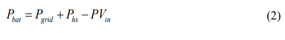
And for the battery acting as a storage system:

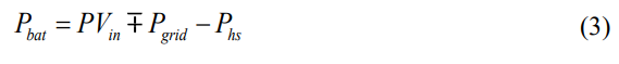
In the first case (Equation 2), the grid may receive injected power or not, depending on the energy balance between the PV array, battery, and household consumption. If the photovoltaic and battery power supply exceeds the household demand, the power injection into the grid is positive; otherwise, it is null. In the second case (Equation 3), the power injection into the grid and the energy storage in the battery depend on the balance between the PV power supply and household energy demand. If the balance is positive, the battery receives the energy surplus as long as it is not completely charged; when this event occurs, the energy surplus is injected into the grid.

Figure 3: Control Unit Operational Flow Chart

Figure 3 shows the operational flowchart that rules the control unit to select the energy flow in the global circuit. The battery charging algorithm is derived from previous work, which enables determining the battery state-of-charge (SOC) through an online process that considers the battery state-of-health (SOH) [57].

Economic Analysis

The energy balance is relevant in decision-making regarding physical battery installation, but it is not the only critical factor. Indeed, economic analysis emerges as a key factor in determining whether the system should equip a physical or virtual battery. Regarding the control unit operational flow chart shown in Figure 3, we notice that the energy flow to the house depends on the household power demand and photovoltaic energy generation, since the energy balance between these two components conditions the battery and grid energy injection or power supply. In current practice, the power injected into the grid depends on factors like the availability of power injection, the maximum compensated power injection, the price paid by the local electric company for the injected power, and the taxes associated with the grid power injection. On the other hand, the cost of energy imported from the grid depends on the electric energy pool, the daily electricity auction, the time of day, and taxes. Considering all these factors, we can base the economic analysis on the following relation: 

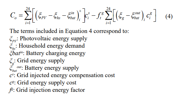
The grid injection energy factor corresponds to the fraction of energy that can be injected according to the regulations of the electric distribution company that operates in the area.

The superscript “+” in Equation 4 means that only the terms with positive contributions are considered for calculation, while we discard null or negative terms. The subscript i corresponds to an hourly interval, since we base the economic analysis on an hourly daily electric energy auction. Equation 4 may require adjustments, depending on country regulations, because the daily electric energy auction may differ from the adopted hourly basis; in such a case, the subscript i corresponds to the new time interval for the electric energy auction. According to the new time interval, we should adjust the summation term.

We observe that the economic balance, C_o, depends on the energy balance and the energy cost. This last term includes the compensation for the injected energy and the payment for the received energy from the grid.

Data Collection

The PV array data collection corresponds to the operating voltage and current measured every second and averaged over a time interval of one minute. We work with a time minute average since a shorter interval does not provide relevant information regarding the system performance evaluation. The control unit uses the voltage and current to determine the PV power generation by applying Ohm’s law. The data collection from the battery block includes the operating voltage, inlet, and outlet current. We use these values to determine the variation in the battery capacity. To this goal, the control unit calculates the battery charge injection or extraction, using the current value and working time. The data correspond to a semidetached three-story house with a total surface of 238 m2, inhabited by a family of four. The house distribution includes a living room, kitchen, toilet, and a small hall on the first floor, four bedrooms and two full bathrooms on the intermediate floor, and an open attic space. A basement used as a garage, with a small room for a workshop, completes the house structure. We obtain the household energy consumption from the appliance power and operating time. Since the working time and power consumption of every appliance are different, we calculate the instantaneous energy consumption through a distribution of built-in energy meters. Since the hourly daily distribution of the household energy consumption changes from day to day, we operate with daily values over a year, computing the energy and economic balance for every day. Electric energy consumption includes lighting, current household electric appliances: entertainment devices, tools and accessories, and an aerothermal energy unit for hot water, heating, and air conditioning.

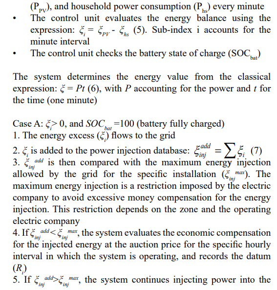
Evaluation Procedure

The evaluation procedure relies on a comprehensive system analysis over an extended period, specifically a whole year, taking into account the aggregate contributions to both the economic and energy balances during this timeframe. The financial aspect, or money balance, serves as the critical factor in determining the suitability of a physical battery. Additionally, the energy balance impacts the size of the physical battery, which in turn affects the overall economic balance. According to the previous statements, we proceed to disaggregate the collected data into four categories: photovoltaic output power, household power consumption, battery input/output power, and grid power injection/supply. The battery and grid categories may act as a power source or sink, depending on the energy balance in the system. Since data collection uses a minute interval base, a non-current time lapse in energy balance for commercial purposes, we use an hourly time basis for economic balance evaluation. Nevertheless, to improve the quality and accuracy of the analysis, we continue operating on a minute- by-minute basis for the energy balance. The evaluation, therefore, uses the following structure (Figure 4):

Figure 4: Schematic View of the Evaluation Process Layout

The battery section on Figure 4 appears shadowed because the physical battery is optional; in case the system operates under virtual battery mode, the physical battery is not part of the layout. grid, but the money compensation is skipped 6. The process continues for the hourly interval, adding the money 60 The evaluation process includes two options: physical battery and virtual battery. Based on this structure, the evaluation procedure is as follows: Option 1: Physical battery • The control unit collects data from the PV array output power

   grid, but the money compensation is skipped

6. The process repeats for the 24 hours in a day, and the 365 days

2. The process continues until the battery is exhausted

3. The control unit engages the grid connection to cover the energy deficit

4. The control unit evaluates the energy price from the grid supply at the setup selling price for the operating time interval, and records the datum

5. The process continues for the hourly interval, adding the calculated price (S_j)

6. The process repeats for the 24 hours in a day, and the 365 days in a year, obtaining the Sy value

1. The control unit engages the grid connection to cover the energy deficit

2. The control unit evaluates the energy price from the grid supply at the setup selling price for the operating time interval, and records the datum

3. The process continues for the hourly interval, adding the calculated price (S_j)

4. The process repeats for the 24 hours in a day, and the 365 days in a year, obtaining the Sy value

Option 2: Virtual battery

• The control unit collects data from the PV array output power (PPV), and household power consumption (Phs) every minute

6. The process continues for the hourly interval, adding the money compensation (R_j)

7. The process repeats for the 24 hours in a day, and the 365 days in a year, obtaining the Ry value. In months with more or fewer than 30 days, the upper index in the summation in d changes accordingly.

1. The control unit engages the grid connection to cover the energy deficit

2. The control unit evaluates the energy price from the grid supply at the setup selling price for the operating time interval, and records the datum

3. The process continues for the hourly interval, adding the calculated price (S_j)

4. The process repeats for the 24 hours in a day, and the 365 days in a year, obtaining the Sy value. In months with more or fewer than 30 days, the upper index in the summation in d changes accordingly

The evaluation process ends by comparing the Sy value for the two options, S_y1 for the physical battery configuration, and S_y2 for the virtual battery mode. If S_y1>S_y2, the physical battery option is recommended; otherwise, the virtual battery mode is the most suitable.

Experimental Development

The methodology mentioned earlier has been tested in an experimental installation, as shown in Figure 1. The system operates according to the following configuration:

• A photovoltaic array of 9 kWp, divided into two sub-arrays of 4.5 kWp. One of the sub-arrays is oriented East, while the other faces West. The PV panels' tilt is 40º (East and West). The two sub-arrays merge in a single inverter. The operating voltage of every sub-array is 360 VDC, with a maximum input current of 12.5 A. Because of the East-West orientation of the PV array, the maximum combined output power is 6.75 kW

• A lithium-ion battery block of 5.04 kWh energy capacity, operating at 360 VDC. The battery layout consists of 10 elements connected in series. Each component has a capacity of 140 Ah operating at 36 VDC.

• An inverter of 7 kW equipped with a double MPPT unit for sub array control. The inverter is a triple-configured unit controlling the PV array, the battery block, and the household connection.

• A household of three stores with conventional appliances and an aerothermal unit for sanitary water, heating, and air conditioning. The aerothermal system's power peak is 6 kW, but it currently operates at a lower power demand, depending on the hot water, heating, and refrigeration requirements.

• An aerothermal system for household sanitary hot water, heating,and air conditioning supply. The aerothermal system operates at a peak power of 6 kW for heating or air conditioning. Hot water supply only requires a maximum power of 5.6 kW

• A control unit that selects the aerothermal unit operational mode,heating or air conditioning, depending on the season of the year, winter or summer Because the use of the aerothermal unit and household appliances and accessories is not regular every day of the year, we have computed the energy consumption, averaging over a week. Since weekly energy consumption changes with the time of the year, we apply the weekly energy use evolution for the entire year. On the other hand, we alternate between heating and air conditioning use; heating operates from October to May, and air conditioning is activated from June to September, which in turn influences the corresponding weekly energy consumption. Regarding the influence of household appliances and accessories on energy use, we notice a regular trend with slight variation from one season to another; therefore, we adopt a uniform evolution of weekly energy consumption throughout the entire year.

Experimental Data

Once we collect the experimental values, we notice the low differences between weekly data for specific periods of the year; therefore, we group values into the following periods:

• Period 1: From 1st of February to 30th of April

• Period 2: From 1st of May to 31st of July

• Period 3: From 1st of August to 31st of October

• Period 4: From 1st of November to 31st of January

The evaluated parameters corresponding to these periods are PV energy supply, household energy consumption, daily energy balance, daily battery supply, remaining battery energy, grid supply, and grid injection. Daily battery supply and battery energy remaining correspond to the physical battery installation option, while grid supply and injection apply for both configurations, physical and virtual battery mode. Energy balance refers to the difference between PV supply and household consumption. Grid injection corresponds to the energy balance surplus, and grid supply to the energy required to compensate for the energy balance deficit.

Figures 5 to 13 display the experimental results for the evaluated parameters during the afore-mentioned periods.

Tables 1 to 9 correspond to the standard deviation in collected data for the parameter’s evolution shown in Figures 5 to 13.

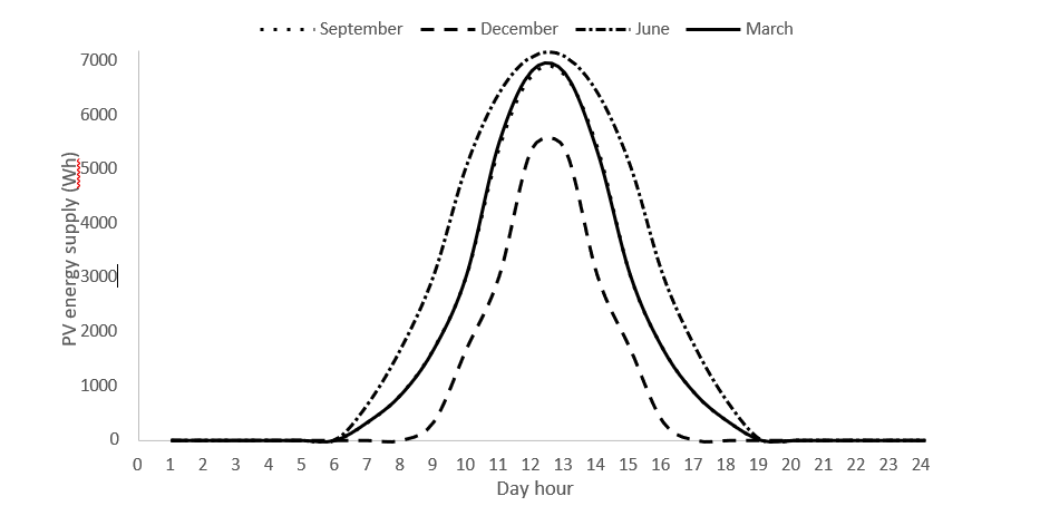
      Figure 5: Daily Pv Energy Supply

Hour	1	2	3	4	5	6	7	8	9	10	11	12
σ(%)	0	0	0	0	0	0	1.7	4.9	4.0	2.7	2.1	3.4
Hour	13	14	15	16	17	18	19	20	21	22	23	24
σ(%)	4.3	3.4	1.2	4.3	2.0	3.0	0	0	0	0	0	0

                                                     Table 1: Average Deviation of Daily Pv Energy Supply

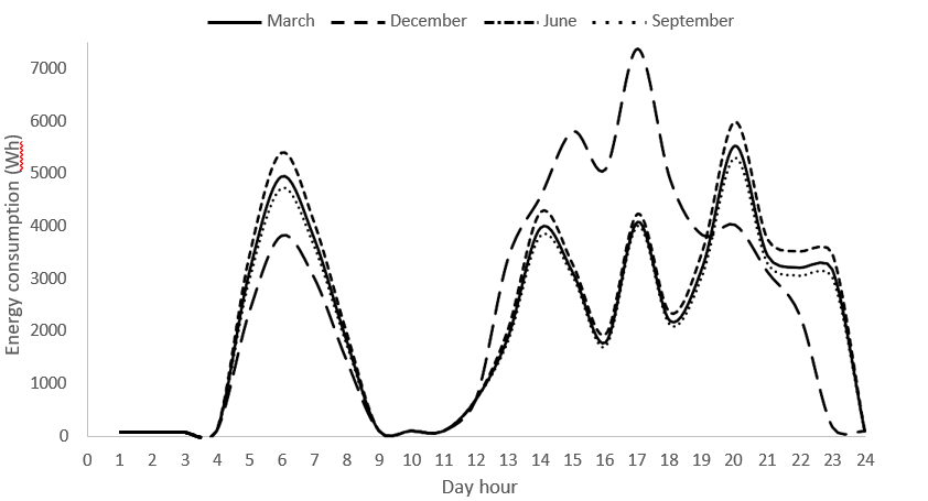
                Figure 6: Daily Household Energy Consumption

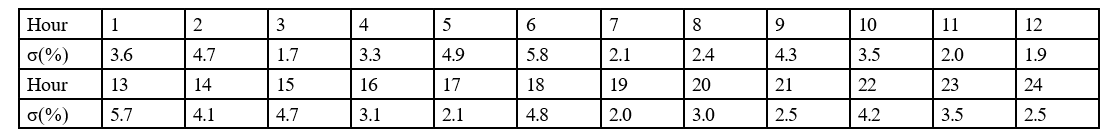
                 Table 2: Average Deviation of Daily Household Energy Consumption

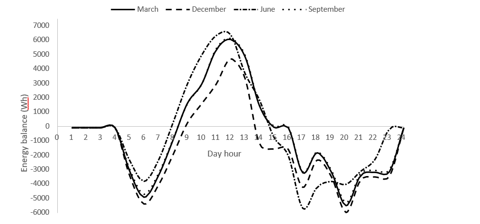
                Figure 7: Daily Energy Balance

Hour	1	2	3	4	5	6	7	8	9	10	11	12
σ(%)	4.6	3.2	1.9	5.9	2.6	5.3	2.7	5.7	4.4	3.3	3.3	5.6
Hour	13	14	15	16	17	18	19	20	21	22	23	24
σ(%)	3.7	5.4	4.8	2.1	2.7	3.1	1.9	5.5	4.9	3.0	3.2	3.5

                                                     Table 3: Average Deviation of Daily Energy Balance

               Figure 8: Daily Battery Supply

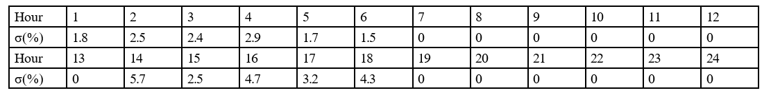
               Table 4: Average Deviation of Daily Battery Supply

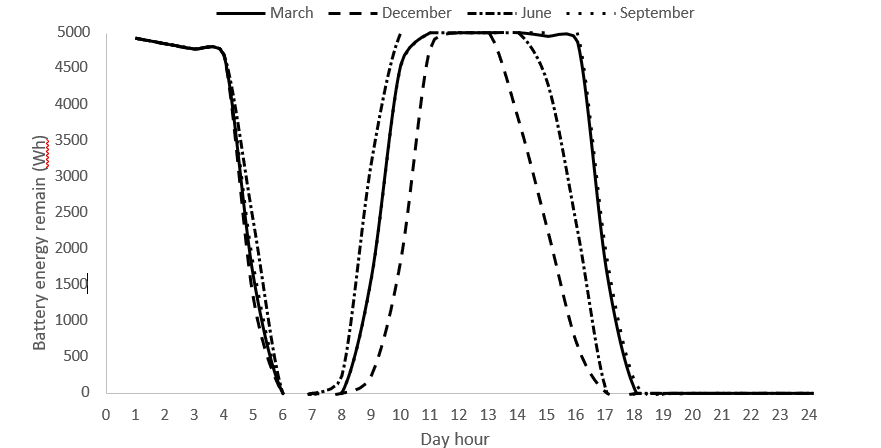
                 Figure 9: Daily Battery Energy Remaining

Hour	1	2	3	4	5	6	7	8	9	10	11	12
σ(%)	4.2	1.8	3.6	2.8	5.1	3.8	3.2	1.5	4.3	2.5	3.6	4.5
Hour	13	14	15	16	17	18	19	20	21	22	23	24
σ(%)	3.0	2.8	3.3	2.1	5.7	0	0	0	0	0	0	0

                           Table 5: Average Deviation of Daily Battery Energy Remaining 

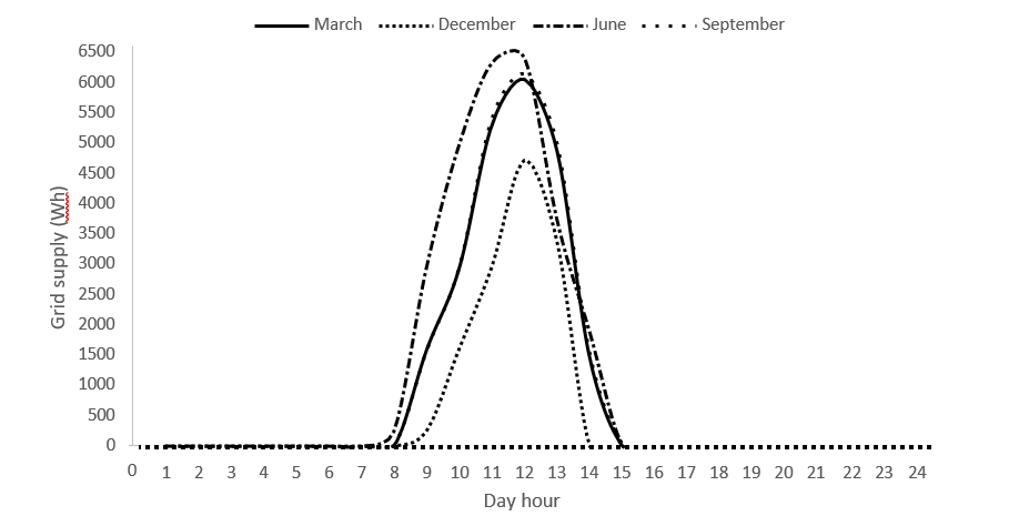
                 Figure 10: Daily Grid Supply (Physical Battery Configuration)

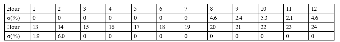
                Table 6: Average Deviation of Daily Grid Supply (Physical Battery Configuration)

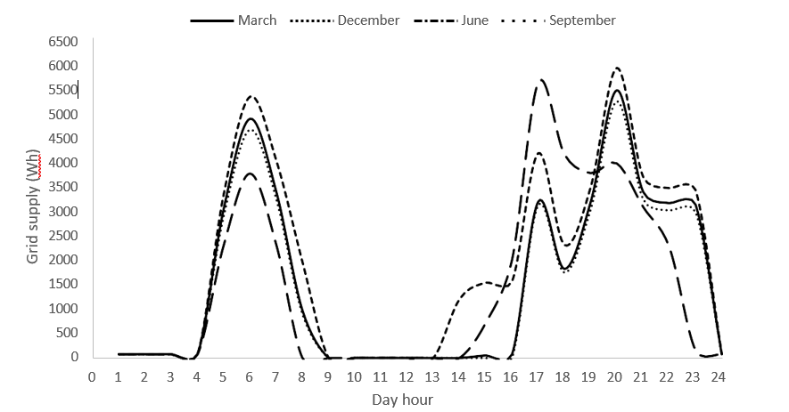
                   Figure 11: Daily Grid Supply (Virtual Battery Configuration)

Hour	1	2	3	4	5	6	7	8	9	10	11	12
σ(%)	1.5	4.3	2.1	3.9	2.1	5.9	2.1	3.9	0	0	0	0
Hour	13	14	15	16	17	18	19	20	21	22	23	24
σ(%)	0	4.9	4.5	6.0	4.5	5.4	4.9	2.2	4.2	5.8	6.0	3.8

                            Table 7: Average Deviation of Daily Grid Supply (Virtual Battery Configuration

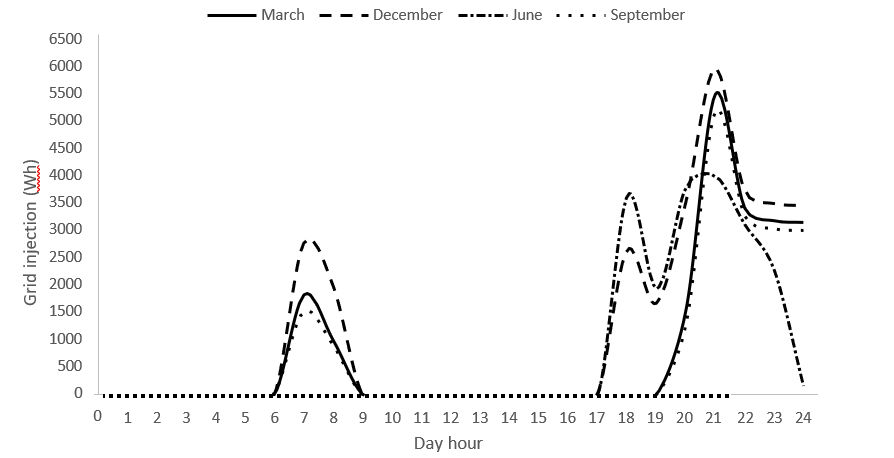
                  Figure 12: Daily Grid Injection (Physical Battery Configuration)

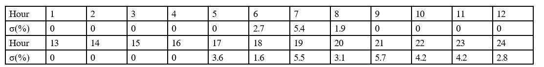
                 Table 8: Average Deviation of Daily Grid Injection (Physical Battery Configuration)

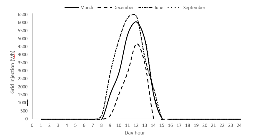
                          Figure 13: Daily Grid Injection (Virtual Battery Configuration)

Hour	1	2	3	4	5	6	7	8	9	10	11	12
σ(%)	0	0	0	0	0	0	0	1.6	1.9	2.7	4.7	3.1
Hour	13	14	15	16	17	18	19	20	21	22	23	24
σ(%)	5.8	3.7	0	0	0	0	0	0	0	0	0	0

                                        Table 9: Average Deviation of Daily Grid Injection (Virtual Battery Configuration)

We notice that all deviations are in the 1.0 to 6.0 range, indicating that all data included in a group remain in a narrow margin around the represented value. The zero values in the deviation refer to null data of the corresponding parameter. Regarding the evaluated parameters, the most interesting analysis corresponds to the comparison between grid supply and injection with physical and virtual battery modes. Indeed, the difference in grid supply and injection indicates the physical battery contribution to the system performance. On the other hand, grid injection depends on the presence or absence of a physical battery and the power supply to the system by said battery. Retrieving values from the database collection, we can obtain the average daily global grid supply and injection data for the physical and virtual battery configurations. Table 10 shows the results for the four periods mentioned before. The values in Table 10 correspond to the representative month of the tested period, as shown in Figures 10 to 13.

	Period 1 March		Period 2         June		Period 3 September		Period 4 December
Battery config.	Physical	Virtual	Physical	Virtual	Physical	Virtual	Physical	Virtual
Grid supply (kWh)	22.274	36.473	26.503	34.808	22.649	34.754	29.235	46.270
Grid injection (kWh)	19.638	22.274	18.945	26.503	18.228	22.526	12.903	12.903
Grid imbalance (kWh)	2.636	14.199	7.558	8.305	4.421	12.228	16.332	33.367

Table 10: Grid Supply and Injection for Physical and Virtual Battery Configuration

We observe that grid supply exceeds grid injection throughout the entire year, regardless of the battery configuration used. This situation indicates a positive imbalance from the grid-to-system, as shown in Table 10 and Figure 14.

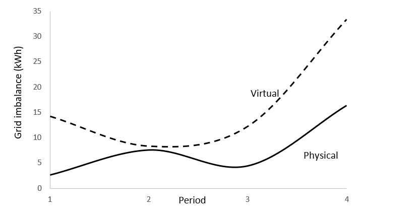
                    Figure 14: Grid-To-System Imbalance for The Tested Periods

We observe that the grid-to-system imbalance nearly matches for physical and virtual battery configuration in period 2 (May through July). This situation shows a low or negligible influence of the battery on the system configuration. On the other hand, in period 1 (February through April), the two curves diverge, showing an increasing difference in the grid-to-system imbalance as we move back from June to March, indicating the influence of the physical battery on the system performance. In periods 3 (August through October) and 4 (November through January), the evolution of the grid-to-system imbalance diverges from August to January, reflecting the influence of the physical battery on the system performance. The physical battery configuration influence on the system performance depends on the grid imbalance difference; the greater the difference, the higher the impact. Therefore, according to data in Table 10, we notice that the maximum influence corresponds to period 4 (November through January), with a grid imbalance difference of 17.035 kWh, and the minimum to period 2, where the grid imbalance is only 0.747 kWh.

Economic Analysis

Using data from Table 10, we may convert the grid imbalance into economic profit or debt. Considering the current price for importing energy from the grid, and the money compensation for grid energy injection, we determine the profit-making balance. In the present case, the current price and money compensation are 0.1815 €/kWh and 0.1 €/kWh; therefore, applying data from Table 10, we obtain (Tables 11 and 12):

Month	January	February	March	April	May	June
Income (€)	87.71	58.91	58.91	58.91	56.84	56.84
Outcome (€)	70.25	121.28	121.28	121.28	144.31	144.31
Balance (€)	17.45	-62.37	-62.37	-62.37	-87.47	-87.47
Month	July	August	September	October	November	December
Income (€)	56.84	54.68	54.68	54.68	87.71	87.71
Outcome (€)	144.31	123.32	123.32	123.32	70.25	70.25
Balance(€)	-87.47	-68.65	-68.65	-68.65	17.45	17.45

Table 11: Economic Balance of Tested Installation (Physical Battery Configuration)

Month	January	February	March	April	May	June
Income (€)	38.71	66.82	66.82	66.82	79.51	79.51
Outcome (€)	251.94	198.59	198.59	198.59	189.53	189.53
Balance (€)	-213.23	-131.77	-131.77	-131.77	-110.02	-110.02
Month	July	August	September	October	November	December
Income (€)	79.51	67.58	67.58	67.58	38.71	38.71
Outcome (€)	189.53	189.24	189.24	189.24	251.94	251.94
Balance(€)	-110.02	-121.66	-121.66	-121.66	-213.23

Table 12: Economic Balance of Tested Installation (Virtual Battery Configuration)

Adding the values for the whole year, we obtain (Table 13):

Battery configuration	Physical	Virtual
Incomes (€)	774.39	757.84
Expenses (€)	1377.49	2487.89
Balance (€)	-603.10	-1730.05

Table 13: Yearly Economic Balance

We observe that in both battery configurations, the economic balance is negative, indicating that we spend more money obtaining energy from the grid than we earn from grid energy injection. Nevertheless, the negative economic balance is higher in the virtual battery configuration, which leads us to recommend using a physical battery for this type of installation. Comparing the yearly economic balance for the two battery configurations, we obtain a monetary profit of 1126.95€. Considering the current cost of a 5-kWh lithium battery unit, around 3365 €, the battery investment payback time is 3 years. Since the expected battery lifespan is 10-20 years, the economic profit may reach up to 13450 €, for a 15-year battery lifespan, and constant current price and compensation money for grid energy supply and injection. The developed economic analysis depends on the current price for energy supply from the grid and economic compensation for grid injection, which is characteristic of every country. The analysis also depends on the battery cost and the need for financing the battery block investment. Since these parameters are variable, it is hard to estimate the battery investment payback time and economic profit under different conditions than those established in the present study. Nevertheless, we have developed a simulation to provide additional data for the final decision-making.

Simulation

The simulation process modifies one of the relevant parameters, keeping all others unchanged. The modified parameter rotates until covering all relevant parameters. Non-relevant parameters remain unchanged during the simulation process. Relevant parameters are battery investment payback time, net economic balance, and grid supply and injection incomes and expenses for physical and virtual battery configurations.

Figure 15 illustrates the battery investment payback time as a function of the battery block investment.

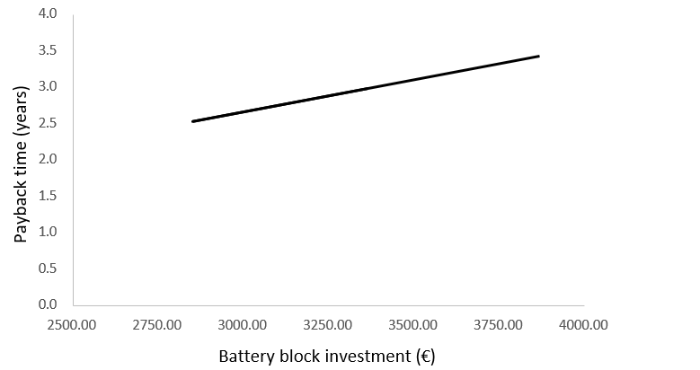
Figure 15: Battery Investment Payback Time vs Battery Cost

We observe a linear dependence between the battery investment payback time and the cost of the battery block, as shown in the Equation PBT = 0.009BI (14), where PBT represents the battery investment payback time and BI represents the price of the battery block. The relationship has a regression coefficient, R² = 1, with a zero error of 10^-14. Equation 14 provides a useful tool to determine the battery investment payback time as a function of any battery block cost. Figures 16 and 17 illustrate the battery investment payback time considering the energy cost supplied by the grid and the grid injection price.

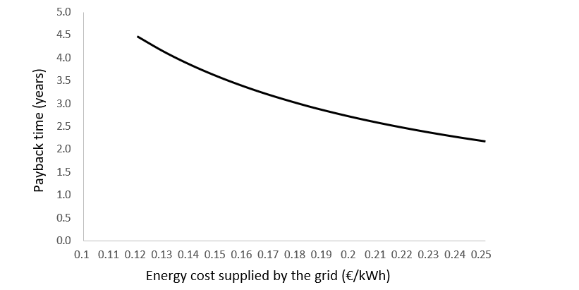
Figure 16: Battery Investment Payback Time vs. Energy Price from Grid Supply

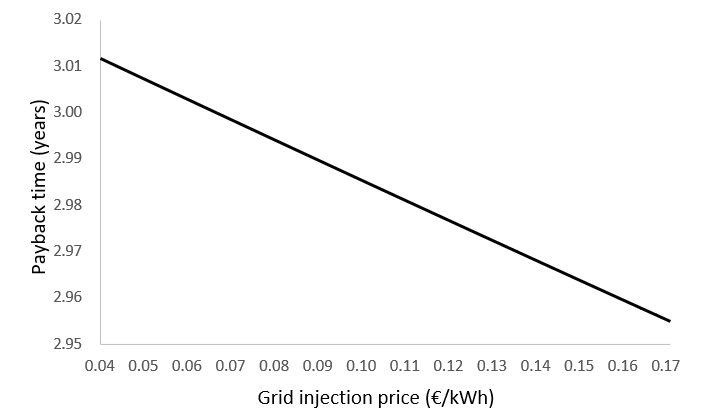
Figure 17: Battery Investment Payback Time vs. Grid Injection Price

Curves in Figures 16 and 17 correspond to the following expressions:

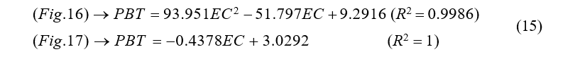
Equation 15 enables installation designers and household users to estimate the battery investment payback time, depending on the energy cost from the grid or the grid injection price.

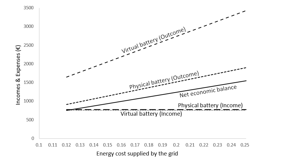
Figure 18: Economic Balance vs. Energy Cost Supplied by the Grid

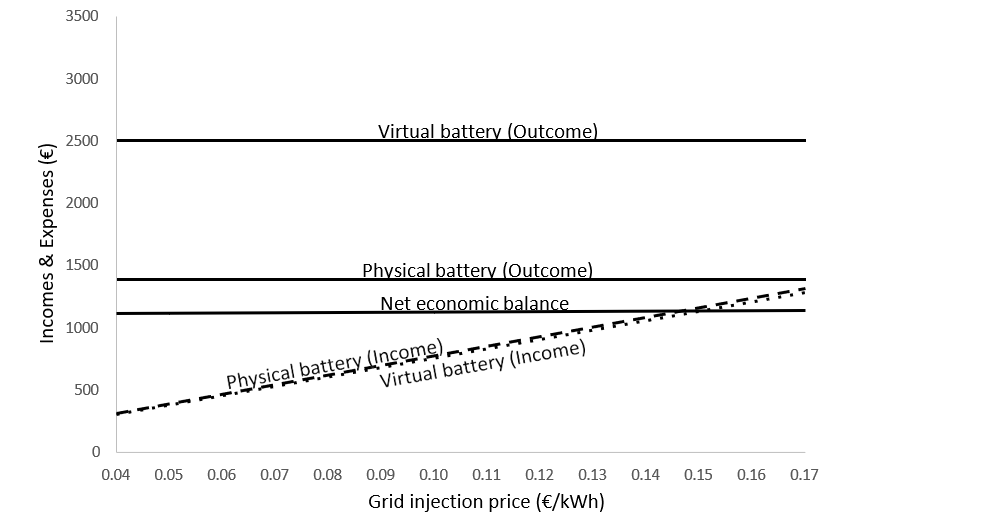
Figure 19: Economic Balance vs. Grid Injection Price

Figures 18 and 19 display the economic balance as a function of the energy cost supplied by the grid and grid injection price.

As expected, the incomes for constant energy cost supplied by the grid remain unchanged for the physical and virtual battery configuration, since there is no dependence between them. A similar situation occurs for the expenses and grid injection price. Regarding the expenses for variable energy cost supplied by the grid and the incomes for variable grid injection price, we observe a linear dependence for both battery configurations (physical and virtual). On the other hand, the net economic balance does not depend on the grid injection price (Figure 19) but increases linearly with the energy cost supplied by the grid (Figure 18); therefore, this last parameter is more influential in the system economic performance than the grid injection price, which shows no influence on it.

Conclusion

Selecting physical or virtual battery configuration for a household installation depends on parameters such as the battery block investment, the energy cost supplied by the grid, and the grid injection price. Among these parameters, the energy cost is the most relevant to the system's economic performance. The grid-to- system energy imbalance, computed as the difference between grid supply and injection to and from the household energy system, shows a low or negligible influence of the battery on the system configuration (physical or virtual) for periods near summer; however, for winter, the influence of the physical battery is high. In year periods like spring and autumn, the physical battery shows an intermediate impact on system energy performance. The economic profit shows that the incomes from a constant energy cost supplied by the grid do not change for both physical and virtual battery configurations, indicating no direct dependence between them. A comparable scenario appears for the outcomes related to grid injection pricing. When examining the expenses, we observe a linear relationship evident for both battery configurations (physical and virtual) concerning variable energy costs from the grid and the incomes influenced by variable grid injection prices. On the other hand, the net economic balance does not depend on the grid injection price but increases linearly with the energy cost supplied by the grid; therefore, this last parameter is more influential in the system economic performance than the grid injection price, showing no influence on it.

References

1. Reports: Approximately 100 million households rely on rooftop solar PV by 2030. Part of Technology and innovation pathways for zero-carbon-ready buildings by 2030. International Energy Agency (IEA).
2. Masson, G., Bosch E., Van Rechem, A., De L’Epine, M. (2024). Snapshot 2024. Technology Collaboration Programme. Photovoltaic Power Systems Programme. International Energy Agency.
3. Watson, J., Sauter, R., Bahaj, B., James, P., Myers, L., & Wing, R. (2008). Domestic micro-generation: Economic, regulatory and policy issues for the UK. Energy Policy, 36(8), 3095-3106.
4. Asano, K., & Aoshima, Y. (2017, November). Effects of local government subsidy on rooftop solar PV in Japan. In 2017 IEEE 6th International Conference on Renewable Energy Research and Applications (ICRERA) (pp. 828-832). IEEE.
5. Sandén, B. A. (2005). The economic and institutional rationale of PV subsidies. Solar energy, 78(2), 137-146.
6. O'Shaughnessy, E. (2022). How policy has shaped the emerging solar photovoltaic installation industry. Energy Policy, 163, 112860.
7. Simpson, G., & Clifton, J. (2016). Subsidies for residential solar photovoltaic energy systems in Western Australia: Distributional, procedural and outcome justice. Renewable and Sustainable Energy Reviews, 65, 262-273.
8. Zhang, Y., Song, J., & Hamori, S. (2011). Impact of subsidy policies on diffusion of photovoltaic power generation. Energy Policy, 39(4), 1958-1964.
9. Hsu, C. W. (2012). Using a system dynamics model to assess the effects of capital subsidies and feed-in tariffs on solar PV installations. Applied energy, 100, 205-217.
10. Borenstein, S. (2017). Private net benefits of residential solar PV: The role of electricity tariffs, tax incentives, and rebates. Journal of the Association of Environmental and Resource Economists, 4(S1), S85-S122.
11. Deng, G., & Newton, P. (2017). Assessing the impact of solar PV on domestic electricity consumption: Exploring the prospect of rebound effects. Energy Policy, 110, 313-324.
12. Strielkowski, W., Štreimikiene, D., & Bilan, Y. (2017). Network charging and residential tariffs: A case of household photovoltaics in the United Kingdom. Renewable and Sustainable Energy Reviews, 77, 461-473.
13. Leonard, M. D., & Michaelides, E. E. (2018). Grid-independent residential buildings with renewable energy sources. Energy, 148, 448-460.
14. Hanser, P., Lueken, R., Gorman, W., Mashal, J., & Group, T.B. (2017). The practicality of distributed PV-battery systems to reduce household grid reliance. Utilities Policy, 46, 22-32.
15. Panapakidis, I. P., Sarafianos, D. N., & Alexiadis, M. C. (2012). Comparative analysis of different grid-independent hybrid power generation systems for a residential load. Renewable and Sustainable Energy Reviews, 16(1), 551-563.
16. Ciocia, A., Amato, A., Di Leo, P., Fichera, S., Malgaroli, G., Spertino, F., & Tzanova, S. (2021). Self-Consumption and self-sufficiency in photovoltaic systems: Effect of grid limitation and storage installation. Energies, 14(6), 1591.
17. Wang, Z., Luther, M. B., Horan, P., Matthews, J., & Liu, C. (2023, October). On-site solar PV generation and use: Self- consumption and self-sufficiency. In Building Simulation (Vol. 16, No. 10, pp. 1835-1849). Beijing: Tsinghua University Press.
18. Nyholm, E., Goop, J., Odenberger, M., & Johnsson, F. (2016). Solar photovoltaic-battery systems in Swedish households– Self-consumption and self-sufficiency. Applied energy, 183, 148-159.
19. Clapes Torres, A. (2021). Viability and design analysis of an energy self-sufficient single-family house disconnected from the electrical grid based on renewable energies (Bachelor's thesis, Universitat Politècnica de Catalunya).
20. Sovacool, B. K. (2009). The intermittency of wind, solar, and renewable electricity generators: Technical barrier or rhetorical excuse?. Utilities policy, 17(3-4), 288-296.
21. Asiaban, S., Kayedpour, N., Samani, A. E., Bozalakov, D.,De Kooning, J. D., Crevecoeur, G., & Vandevelde, L. (2021). Wind and solar intermittency and the associated integration challenges: A comprehensive review including the status in the Belgian power system. Energies, 14(9), 2630.
22. Zhou, S., Wang, Y., Zhou, Y., Clarke, L. E., & Edmonds, J.A. (2018). Roles of wind and solar energy in China’s power sector: Implications of intermittency constraints. Applied energy, 213, 22-30.
23. Mlilo, N., Brown, J., & Ahfock, T. (2021). Impact of intermittent renewable energy generation penetration on the power system networks–A review. Technology and Economics of Smart Grids and Sustainable Energy, 6(1), 25.
24. Denholm, P., & Margolis, R. M. (2007). Evaluating the limits of solar photovoltaics (PV) in traditional electric power systems. Energy policy, 35(5), 2852-2861.
25. Luthander, R., Widén, J., Nilsson, D., & Palm, J. (2015). Photovoltaic self-consumption in buildings: A review. Applied energy, 142, 80-94.
26. Castillo-Cagigal, M., Caamaño-Martín, E., Matallanas, E., Masa-Bote, D., Gutiérrez, Á., Monasterio-Huelin, F., & Jiménez-Leube, J. (2011). PV self-consumption optimization with storage and Active DSM for the residential sector. Solar energy, 85(9), 2338-2348.
27. Gagliano, A., Nocera, F., & Tina, G. (2020). Performances and economic analysis of small photovoltaic–electricity energy storage system for residential applications. Energy & Environment, 31(1), 155-175.
28. Sarasa-Maestro, C. J., Dufo-López, R., & Bernal-Agustín, J.L. (2016). Analysis of photovoltaic self-consumption systems.Energies, 9(9), 681.
29. Vieira, F. M., Moura, P. S., & de Almeida, A. T. (2017). Energy storage system for self-consumption of photovoltaic energy in residential zero energy buildings. Renewable energy, 103, 308-320.
30. Nyholm, E., Goop, J., Odenberger, M., & Johnsson, F. (2016). Solar photovoltaic-battery systems in Swedish households– Self-consumption and self-sufficiency. Applied energy, 183, 148-159.
31. Schram, W. L., Lampropoulos, I., & van Sark, W. G. (2018). Photovoltaic systems coupled with batteries that are optimally sized for household self-consumption: Assessment of peak shaving potential. Applied energy, 223, 69-81.
32. Solar System Without Battery: A Comprehensive Guide. Posted on March 11, 2025.
33. Can I Use Solar Pannels Without Battery Storage? Solar Learning Center. https://www.aforenergy.com/solar-system- without-battery-a-comprehensive-guide/.
34. Meuris, M., Lodewijks, P., Ponnette, R., Meinke�Hubeny, F., Valkering, P., Belmans, R., & Poortmans, J. (2019). Managing PV power injection and storage, enabling a larger direct consumption of renewable energy: A case study for the Belgian electricity system. Progress in Photovoltaics: Research and Applications, 27(11), 905-917.
35. Braun, M., Stetz, T., Bründlinger, R., Mayr, C., Ogimoto, K., Hatta, H., ... & MacGill, I. (2012). Is the distribution grid ready to accept large-scale photovoltaic deployment? State of the art, progress, and future prospects. Progress in photovoltaics: Research and applications, 20(6), 681-697.
36. Ehara, T. (2009). Overcoming PV grid issues in the urban areas.
37. Sechilariu, M., Wang, B., & Locment, F. (2013). Building- integrated microgrid: Advanced local energy management for forthcoming smart power grid communication. Energy and Buildings, 59, 236-243.
38. Pillai, G. G., Putrus, G. A., Georgitsioti, T., & Pearsall, N.M. (2014). Near-term economic benefits from grid-connectedresidential PV (photovoltaic) systems. Energy, 68, 832-843.
39. Cucchiella, F., D’Adamo, I., & Gastaldi, M. (2017). Economic analysis of a photovoltaic system: A resource for residential households. Energies, 10(6), 814.
40. Mondol, J. D., Yohanis, Y. G., & Norton, B. (2009). Optimising the economic viability of grid-connected photovoltaic systems. Applied Energy, 86(7-8), 985-999.
41. Colmenar-Santos, A., Campíñez-Romero, S., Pérez-Molina, C., & Castro-Gil, M. (2012). Profitability analysis of grid- connected photovoltaic facilities for household electricity self-sufficiency. Energy Policy, 51, 749-764.
42. Fernández-Infantes, A., Contreras, J., & Bernal-Agustín, J.L. (2006). Design of grid connected PV systems considering electrical, economical and environmental aspects: A practical case. Renewable Energy, 31(13), 2042-2062.
43. Payment for service and goods (e.g. Feed-in tariff, Electricity capacity remuneration mechanisms). United Nations Climate Change.
44. Camilo, F. M., Castro, R., Almeida, M. E., & Pires, V. F. (2017). Economic assessment of residential PV systems with self-consumption and storage in Portugal. Solar Energy, 150, 353-362.
45. What is the compensation for solar panels consumption surpluses? Energy explained, Green Energy, Saving Energy. Energy Nordic. Last updated on May 9, 2025.
46. Wang, R., Hasanefendic, S., Von Hauff, E., & Bossink, B. (2022). The cost of photovoltaics: Re-evaluating grid parity for PV systems in China. Renewable Energy, 194, 469-481.
47. Kiso, T., Chan, H. R., & Arino, Y. (2022). Contrasting effects of electricity prices on retrofit and new-build installations of solar PV: Fukushima as a natural experiment. Journal of Environmental Economics and Management, 115, 102685.
48. Yamamoto, Y. (2012). Pricing electricity from residential photovoltaic systems: A comparison of feed-in tariffs, net metering, and net purchase and sale. Solar energy, 86(9), 2678-2685.
49. Debruyne, C., Desmet, J., Vanalme, J., Verhelst, B., Vanalme, G., & Vandevelde, L. (2010). Maximum power injection acceptance in a residential area. In International Conference on Renewable Energies and Power Quality (ICREPQ 2010). European Association for the Development of Renewable Energies, Environment and Power Quality.
50. Lucas, A. (2018). Single-phase PV power injection limit due to voltage unbalances applied to an urban reference network using real-time simulation. Applied Sciences, 8(8), 1333.
51. Ruf, H. (2018). Limitations for the feed-in power of residential photovoltaic systems in Germany–An overview of the regulatory framework. Solar Energy, 159, 588-600.
52. Hoppmann, J., Volland, J., Schmidt, T. S., & Hoffmann, V. H. (2014). The economic viability of battery storage for residential solar photovoltaic systems–A review and a simulation model. Renewable and Sustainable Energy Reviews, 39, 1101-1118.
53. Uddin, K., Gough, R., Radcliffe, J., Marco, J., & Jennings,P. (2017). Techno-economic analysis of the viability of residential photovoltaic systems using lithium-ion batteries for energy storage in the United Kingdom. Applied energy, 206, 12-21.
54. Cristea, C., Cristea, M., Birou, I., & Tîrnovan, R. A. (2020, May). Techno-economic evaluation of a grid-connected residential rooftop photovoltaic system with battery energy storage system: a Romanian case study. In 2020 International Conference on Development and Application Systems (DAS) (pp. 44-48). IEEE.
55. Xiong, L., & Nour, M. (2019). Techno-economic analysis of a residential PV-storage model in a distribution network. Energies, 12(16), 3062.
56. Nkuriyingoma, O., Özdemir, E., & Sezen, S. (2022). Techno- economic analysis of a PV system with a battery energy storage system for small households: A case study in Rwanda. Frontiers in Energy Research, 10, 957564.
57. Armenta-Déu, C. (2025). Online determination of State of Health (SOH) in Lithium-ion Batteries: Influence of aging on the State of Charge. Frontiers in Research Energy. 13:1573972.