Typical Weather Year for the Design of Thermal Applications in Social Housing

Introduction

The global trend of world energy consumption in recent years has been primarily based on the consumption of hydrocarbons.Although social awareness of climate change seems to be well established, the push from emerging countries has resulted in the adoption of renewable technologies being much lower than expected in favor of conventional energy usage. Currently, there are 37-member countries of the OECD (Organization for Economic Cooperation and Development), of which 20 are founders and the rest have joined successively. The EU has observer status in the Council with voice but without vote. In addition to the OECD member states, 11 non-member countries have signed the implementation of the OECD Guidelines: Argentina, Brazil, Costa Rica, Egypt, Jordan, Morocco, Peru, Romania, and Tunisia. Furthermore, the OECD maintains a closer and more privileged relationship with the so- called Key Partners (Brazil, China, India, Indonesia, and South Africa) who even participate in Ministerial Meetings. According to the report of the US Energy Information Administration, global energy consumption will increase almost 50% between 2018 and 2050 [1]. Almost all of the increase occurs in non-OECD countries. Most of the increases in energy consumption come from non-OECD countries where strong economic growth, greater access to commercial energy, and rapid population growth lead to increased energy consumption. In OECD countries, energy consumption growth is slower due to relatively slower population and economic growth, improvements in energy efficiency, and less growth in energy-intensive industries. Energy consumption in non-OECD countries increases by almost 70% between 2018 and 2050, compared to a 15% increase in OECD countries.

Energy consumption in the building sector, which includes residential and commercial structures, increases by 1.3% per year, a growth rate higher than the annual world population growth, from 91 quadrillion to 139 quadrillion British thermal units (BTUs) from 2018 to 2050. The share of the building sector in global supplied energy consumption increases from around 20% in 2018 to 22% in  2050 [1]. Most of the increase in energy use comes from countries that are not part of the Organization for Economic Cooperation and Development (OECD). These countries are experiencing rising incomes, urbanization, and greater access to electricity, leading to higher energy demand. Building energy consumption in non- OECD countries increases by approximately 2% per year, about five times faster than in OECD countries, and non-OECD building energy consumption will surpass that of OECD countries by 2025.

In OECD countries, building energy consumption is projected to increase at an average annual rate of 0.4% from 2018 to 2050, reflecting slow personal income growth and energy efficiency gains resulting from improved building structures, appliances, and equipment. Global residential energy consumption per person (energy intensity) increases by 0.6% per year from 2018 to 2050, as residential energy consumption (1.4% per year) grows faster than the global population growth (0.7% per year). In OECD countries, residential energy intensity decreases by an average of 0.1% per year from 2018 to 2050, compared to an average increase of 1.3% per year in non-OECD countries over the same period. India experiences the fastest relative growth in residential energy use per person due to greater access to energy sources and increased use of appliances and other energy-consuming equipment. However, in 2050, India's per-person residential energy use is only about 24% of that in the United States. Although residential energy intensity in Africa grows by about 16% between 2018 and 2050, it remains the least energy-intensive region. Electricity continues to be the main source of commercialized energy consumption in the residential sector, and its use grows by 2.5% annually worldwide as the population and living standards increase in non- OECD countries, driving the demand for appliances and personal equipment. Residential natural gas consumption increases by 0.7% annually during the projection period, influenced by the growing use of natural gas for heating. Coal consumption, mainly used for space heating, water heating, and cooking, continues to decline in the residential sector. Globally, the amount of energy used per unit of economic output (energy intensity) has steadily decreased over many years. In OECD countries, projected energy-related CO₂ emissions decrease slightly (-0.2% per year) until 2050 and are 14% lower than their 2005 levels in 2050, even as their economies gradually expand. Energy-related CO₂ emissions in non-OECD countries grow at a rate of around 1% per year between 2018 and 2050, slower than the related growth in energy consumption (1.6% per year).

Lifestyle also has a clear impact. In a situation of prosperity, there is greater consumption and/or little care in the rational use of resources. This results in increased resource use, waste generation, and ultimately CO₂ production. "Buildings, essential for life and consumption, could reduce adverse ecological effects through better design that considers sustainability" ..."Architecture alone cannot solve the planet's environmental problems, but it can significantly contribute to the creation of more sustainable human habitats" [2]. Having complete and accurate meteorological information is crucial for obtaining reliable results in Building Energy Simulation. It is necessary to know various meteorological parameters such as dry bulb temperature, relative humidity, wind speed and direction, atmospheric pressure, solar radiation, etc., that are representative of the climate in the location where the building is or will be constructed or improved if it already exists. More sophisticatedly, ASHRAE (American Society of Heating, Refrigerating and Air- Conditioning Engineers) uses models that allow reconstructing the variation of the parameters of interest over the 24 hours of a typical seasonal or monthly day [3]. The thermal response of a building on any given day generally depends on the weather conditions of the previous day, an effect that is impossible to capture using the typical monthly or seasonal day concept. Therefore, it is necessary to have continuous meteorological information throughout all seasons, that is, over an entire year considered representative of the location. Such information can be organized in various ways, with the concept of a Typical Meteorological Year (TMY) introduced by Hall et al. being chosen here [4]. A TMY is a set of hourly meteorological data that represents the weather conditions considered typical for a given location over a relatively long period. This article designs a TMY for use in building energy simulations. It will be applied to the design of a social housing unit to detail the energy requirements for both heating and cooling.

    Bioenvironmental

Zones The bioenvironmental zones are defined according to the map in Figure 1. This classification has been developed considering the effective corrected temperature comfort indices (TEC), correlated with the predicted mean vote (PMV) and the Belding and Hatch index (BHI), developed for warm zones. The evaluation of cold zones has not been performed using comfort indices but rather degree days for heating needs.

Corrected effective temperature (CET) values were used exclu- sively for the purpose of the bioenvironmental classification. These values should not be used to carry out thermal balances aimed at sizing air conditioning installations. For this purpose, the dry bulb temperature and relative humidity or wet bulb temperature values for typical design days should be used [5].

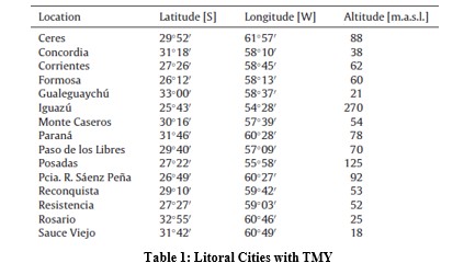
     TMY in Argentina

In our country, few locations have their TMY. Bre et al. describe the generation of the typical meteorological year for 15 locations throughout the Litoral Region in northeastern Argentina (Table 1) [6]. The author obtains available meteorological data at each site, including dry bulb temperatures, dew point temperatures, wind speed, and total sky cover, measured hourly during the period 1994-2014 by the National Meteorological Service (NM) of Argentina. Two of these locations only have hourly solar radiation data for some years. These radiation measurements were used to calibrate an existing Zhang-Huang solar radiation model, which was then used to compute hourly solar radiation for the entire meteorological database.

For the development of the TMY for the city of Santa Fe, Bre et al. used the climatic file corresponding to the Brazilian city of Uruguaiana, the closest known typical year of climatic conditions to those of Santa Fe city [7, 8]. The TMY of Santa Fe city was defined based on data provided by the National Meteorological Service (SMN) of Argentina, recorded at Sauce Viejo Airport during the period 2000-2013. The data provided by the SMN does not include Global Solar Radiation (GSR), a variable of utmost importance for defining the TMY. Therefore, the authors resorted to GSR data provided by the Meteorological Information Center (CIM) of the Faculty of Engineering and Water Sciences (FICH) of the National University of the Litoral (UNL). These data were recorded on the Faculty campus, located in the University City of UNL, in Santa Fe city. The data were recorded every 10 to 15 minutes during the period from October 2008 to April 2014. Unfortunately, the GSR data from CIM were not sufficiently complete to be directly included in a statistical analysis. For this reason, they decided to calculate the GSR using the model, and use the most complete year registered by to validate the model and obtain new adjustment parameters. The same procedure was applied to generate the TMY for the city of La Plata [9-11]. Finally, the Autonomous City of Buenos Aires (CABA) has its TMY defined [12].

        Climatic Characteristics of the City of Salta

The city of Salta (1,232 meters above sea level), capital of the province of the same name, is located in bioenvironmental zone III, Subzone IIIa [5]. This zone is warm-temperate, bounded by the TEC (Corrected Effective Temperature) isolines of 24.6 °C and

22.9 °C. This zone has the same distribution as zone II, with an East-West extension strip centered around the 35° parallel and a North-South extension strip located in the first mountain foothills in the Northeast of the country, on the Andes mountain range. Summers are relatively hot, with average temperatures between 20 °C and 26 °C, and average highs exceeding 30 °C only in the East-West extension strip. Winter is not very cold, with average temperature values between 8 °C and 12 °C, and minimum values rarely dropping below 0 °C. The partial vapor pressures are low throughout the year, with maximum values in summer not averaging more than 1870 Pa (14 mm Hg). Generally, this zone experiences relatively mild winters and moderately hot summers. This zone is subdivided into two subzones: a and b, based on thermal amplitudes.

• • • Subzone IIIa: thermal amplitudes greater than 14 °C.
    • Subzone IIIb: thermal amplitudes less than 14 °C.

         TRY, TMY, TMY2, TMY3 y IWEC

Currently, there are two common types of typical meteorological data adopted for building energy simulations: The Test Year of Reference (TRY) and the Typical Meteorological Year (TMY). In a TRY, the 8,760-hour climatic information for a particular year is selected by a simple procedure established by the American Society of Heating, Refrigerating, and Air-Conditioning Engineers [13,14]. Throughout the selection process, only one climatic index is adopted, namely the dry bulb temperature. All candidate months within the study period are classified, alternating between the hot half (November-April) and the cold half (May-October) of the year. The extreme months are ordered by the average monthly dry bulb temperature. A TRY is selected by eliminating candidate years within the study period that contain months with extremely high or low dry bulb temperatures. The elimination process is continued until only one year remains, which is the selected TRY.

During the selection of TRY, candidate months with extremely high or low monthly dry bulb temperatures are progressively eliminated, resulting in a particularly mild year that may not represent the typical long-term climatic condition. Constructing energy simulations using meteorological data from the TRY is obviously less reliable in reproducing average historical conditions [15]. TRY weather data tapes were originally developed by the US National Climatic Data Center for research purposes. ASHRAE stated that the TRY is not recommended for medium to long-term studies of building performance [16]. The German weather service (DWD) and the Dutch weather service have conducted multiple studies regarding the update and improvement of TRYs. The DWD has TRYs covering more than ten parameters and methodologies for calculating TRYs for extreme years.

TMY is another common type of meteorological data widely adopted by various researchers. As mentioned earlier, a set of TMY data provides full-year meteorological data representing the climatic conditions in a specific city over a reasonably long period. The selection of a TMY uses data from nine critical climatic indices, including daily maximum, minimum, and average dry bulb and dew point temperatures; daily maximum and average wind speed; and total daily global horizontal solar radiation.

For the TMY selection procedure, TMY meteorological data sets were developed for 26 SOLMET stations in the U.S. (known as the Sandia method) [5]. In 1994, the National Solar Radiation Database (NSRDB) followed the Sandia method with modified weighting factors (Table 1) to generate 239 TMY data sets for a series of weather stations in the United States [17]. This new set of TMY meteorological data was labeled as TMY2. Similarly, a set of TMY weather files was produced by ASHRAE in 1997 by using another set of new weighting factor for the climatic indices used in the Sandia method [18]. This data set, referred to as the International Weather for Energy Calculation (IWEC), contains hourly TMY weather files for 227 cities in over 70 different countries. In 2007, a new set of TMY meteorological data (titled TMY3) was generated by the National Renewable Energy Laboratory (NREL) [19]. These TMY3 weather files provide updated meteorological data with greater coverage of over 1000 locations in the United States. In this article, a typical meteorological year was developed using a method that combines the weighting factors of the TMY- generating sets mentioned above. The method was named TMY Plus.

     TMYs in the World

To model and study the dispersion of pollutants in the atmosphere, long-term data is generally adopted (known as the classical approach). In Italy, they explored the possibility of using a TMY generated with a new set of weighting factors (10/16 for mean wind vspeed, 5/16 for global radiation, and 1/16 for mean temperature), which was evaluated through a pairwise comparison method with the participation of a group of experts [20]. The result of the simulation using the new TMY weather file demonstrated good agreement with the results obtained through multi-year simulation of 10-year data. Typical meteorological years for eight cities with different climates in China were generated by Jiang using available meteorological data from the period 1995-2004 and the Sandia method [21]. Based on the authors' judgment, relatively large weighting factors of 0.5 (0.25 for global solar radiation and 0.25 for direct solar radiation) and 0.25 (for dry bulb temperature) were assigned. The reason is that solar radiation and dry bulb temperature represent a significant part of the building's cooling load, and other climatic indices are more or less dependent on the amount of solar radiation. In Nigeria, typical meteorological years for five different locations were developed by [22].

The authors intuitively assigned weighting factor values for the main meteorological parameters. Weighting factors of 5/12 and 2/12 were assigned to global solar radiation and mean dry bulb temperature, respectively, while the other meteorological parameters were given equal weighting factors adding up to 5/12. These TMYs were generated mainly for application in solar energy systems. In the study by, the Sandia method was applied to select typical meteorological data for Subang, Malaysia, with six sets of arbitrarily assigned weighting factors for four meteorological parameters [23]. The study revealed that typical meteorologicalvdata selected using equal weighting factors were suitable for constructing energy simulations, unless there were reasons to use another combination of weighting factor for selecting typical meteorological data for application in other energy systems. Author A.L.S. Chan developed a new weather file generator using genetic algorithms (GA) [24]. By employing this weather file generator, optimal sets of weighting factors can be generated to develop appropriate TMY files for different energy systems. Previous studies conducted by various researchers conclude that a set of correct weighting factors plays a crucial role in generating appropriate TMY weather files for the computational simulation of different applications. However, there is no fundamental principle or general agreement on the assignment of weighting factor values to climatic factors in the generation of TMYs.

Materials and Methods

    Weighting Factors

The weighting factor values of the climatic indices used in the Sandia method play an important role in the TMY generation process. These weighting factors express the relative importance of the impact of a particular climatic index on the thermal and energy performance of a building or an energy system. Various sets of weighting factors have been adopted by different researchers. The ones used in this thesis are detailed in Table 2. The values of these weighting factors were primarily assigned based on the researcher's experience regarding the influence of the climatic indices on thermal performance.

                                          Table 2: Sets of Weighting Factors for Various Climate Indices.

To cite some previous research works conducted by researchers on this topic, developed a typical meteorological year for the Argentine coastal region using the Hall method, commonly called TMY1 [7]. Yang and Lu investigated the effect of the typical meteorological year (TMY) and the example weather year (EWY) on the energy simulation results of buildings and solar- wind hybrids [25]. According to the authors' previous experience and academic judgment, high weightings were assigned to solar radiation and wind speed (11/24 for each) to generate a TMY. A computer simulation was conducted to evaluate the energy performance of a solar-wind hybrid energy system using the TMY weather file generated by the authors. The result showed that, for the solar-wind hybrid energy system, a maximum difference of 20% could be found in the simulation result compared to the simulated output using a TMY weather file generated with Hall's original weighting factors, concluding that the EWY method is not appropriate for representing the annual weather file.

Typical Meteorological Month TMM Selection Procedures

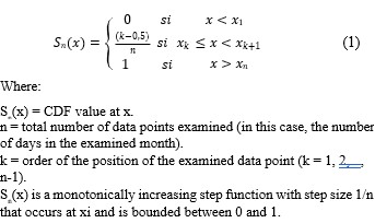
In this chapter, the development of the TMY weather data file basically follows the selection procedures of the Sandia TMY, TMY2, IWEC, CHAN, and TMYPlus methods. In all five methods, nine critical climatic indices including daily maximum, minimum, and average dry bulb and dew point temperatures; daily maximum and average wind speed; and total daily global horizontal solar radiation are evaluated using the Finkelstein-Shafer (FS) statistics to select 12 TMM. For each candidate month in each individual year, the cumulative distribution function (CDF) for each of the nine climatic indices is determined. The CDF for each climatic index x is defined as follows in equation (1):

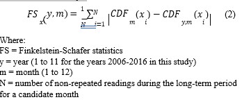
Using the same equation, Equation (1), the long-term CDF values covering the entire study period are also evaluated. The Equation (2) shown below is used to calculate the absolute difference (FS statistic) between the short-term CDF of a candidate month in an individual year and the long-term CDF to measure the degree of closeness or similarity.

                          Table 3: Finkelstein-Schafer Statistics from January to May 2006.

As an example of the procedure, Table 3 details the climatological indices with the Finkelstein-Schafer statistics for each one corresponding to the months from January to May of the year 2006. To reflect the relative importance of each climatic index in the selection of the TMM, a set of weighting factors (WF) is applied to calculate a weighted sum (WS) of the FS statistics, expressed in Equation (3). A summary of the weighting factors for the nine climatic indices is listed in Table 2. In this development of the TMYPLUS, the four sets of weighting factors were used.

Table 4: Weighted Sum for Each Climate Index for January 2006.

In Table 4, each column is the result of applying Equation (3), while the last row is the weighted sum (WS) of each TMY  developer, all corresponding to January 2006. The same procedure is subsequently carried out for each month of each sample year. The WS values are calculated for each candidate month of each individual year. Then all months are ranked in ascending order according to their WS values. For each month, five candidate months with the lowest WS values are selected for further selection.

In the Sandia method, a persistence structure is incorporated in order to exclude candidate months with the longest (number of days) or shortest months. Fixed percentiles for the long-term will be evaluated for the frequency and duration of the mean dry-bulb temperature and total daily solar radiation, serving as additional criteria for selecting a TMM from the previously identified five candidate months (with the lowest WS values). However, IWEC (ASHRAE, 2002) noted that the five candidate months with the lowest WS values could be rejected by the persistence structure criterion in the final selection stage implemented by the Sandia method. In the present study, the IWEC recommendation was followed, and the persistence structure was not adopted. The candidate month with the lowest WS value was identified as the TMM, as the weighted sum WS indicates how far I am from the long-term mean analyzed (in this case, 11 years of data). The weighted sum (WS) values of the FS statistics for each candidate month (Jan-Dec) of the 11-year period (2006-2016) are tabulated in Table 5 and Table 6. As indicated, the WS values printed in bold and underlined identify the candidate TMMs for each method.

Typical Meteorological Year in Salta (TMYPlus)

For the development of TMYPLUS, the selection of the candidate TMM was performed by applying five different methods for generating TMY. The first method is the so-called TMY1, whose weighting factors are shown in Table 2, similarly for the other methods; TMY2 and TMY3; IWEC, and the method generated with the Generic Algorithm (GA) by the author Chan [4,17,18,24]. The fifth method is a combination of the weighting factors of the four sets of WFs that make up the methods. This method, as mentioned, is TMYPlus, which is ultimately applied to select the TMM from our final meteorological file.

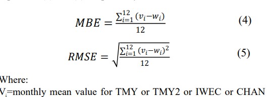
To have a quantitative comparison between these five profiles, the mean bias error (MBE) and the root mean square error (RMSE) values were calculated for these five TMYs against the 11-year average. Based on these errors, the optimal set of weighting factors for their respective climatic indices that make up TMYPlus was selected. The definitions of MBE and RMSE are expressed in Equations (4) and (5), respectively.

Data Description

To characterize the typical meteorological conditions in the city of Salta (Lat. -24.7°, Long. -65.5° and 1232 masl), we used data provided by the National Meteorological Service (SMN), recorded between 2006 and 2016 by the Martin Miguel de Güemes International Airport and the Institute for Energy Research and Non-Conventional Energy (INENCO). The recorded variables are: Global Horizontal Solar Radiation, Dry-Bulb Temperature, Dew Point Temperature, Wet-Bulb Temperature, Wind Direction, Wind Speed, Atmospheric Pressure, and Relative Humidity. Typically, the interval between SMN records is one hour, while the radiation data was measured every 15 minutes and consists of at least 11 years of data. The radiation measurements were taken with a KIPP ZONEN CM3 pyranometer by researcher Ricardo Echazú from INENCO.

Building Energy Simulation Program

To study the indoor air and wall surface temperatures, energy consumption, and comfort conditions, the software SIMEDIF Version 2.0 is used. This program is developed by researchers at INENCO and is freely available at INENCO – Institute for Energy Research and Non-Conventional Energy (unsa.edu.ar). SIMEDIF is a design tool used to calculate the hourly air temperature within building spaces, the hourly surface temperature of walls, and the auxiliary heating/cooling energy needed to maintain spaces at a temperature determined by a thermostat, which can be defined hour by hour for the entire year.

The program allows analyzing the building's behavior under different climatic conditions, detecting thermal comfort issues (overheating or low temperatures), and evaluating possible design alternatives for a building, such as changes in its geometry, orientation, location, and size of the building, the structure and materials of the envelope, the addition of passive and hybrid systems like earth-air coolers, evaporative coolers, double green facades, etc. In existing buildings, the software can be used to validate the construction model through measured data or to quantify the effectiveness of possible redesign alternatives in the case of energy rehabilitation [26].

This Windows version was developed by Dr. Silvana Flores Larsen at INENCO (Institute for Non-Conventional Energy Research, U.N.Sa.-CONICET). The original 1984 DOS version was developed by Drs. Graciela Lesino, Luis Saravia, and Dolores Alía. The current version consists of two parts: data entry (made with VisualBasic 6) and the calculation module (entirely developed in Python). The data entry is completely transparent (plain text files), so any programmer can develop their own input interface if required. More details of the thermal model can be found in [27].

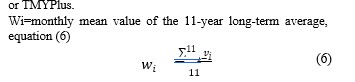
Description of Social Housing

Simulations will be conducted for extreme winter and summer conditions of a social housing unit for a typical family, such homes are delivered here in the city of Salta. It will be simulated with the typical meteorological year (TMYPlus) generated in this article. The house has a built area of 63.7 m². It consists of three rooms, a kitchen-dining room, and a bathroom, as shown in Figure 2. The vertical envelope is made of hollow ceramic brick 0.18 m thick  with coarse and fine lime plaster on both sides, with a thickness of 0.01 m, without thermal insulation. The horizontal envelope is a sloping roof composed of a suspended gypsum board ceiling of 9.5 x10^-3 m thickness, located 2.6 m above the ground. Above the ceiling, there is an air chamber after which there is a 25-gauge sheet metal (5 x10^-4 m thickness). The ceiling is attached to the sheet metal with "C" profile fixing straps.

While data entry can be performed in any order for the elements, the first step is, necessarily, to define the location and climate. We chose to simulate the city of Salta Capital. In the Climate selection part, we will choose the TMYPlus created in this article. It is in .epw format. The .epw format (EnergyPlus Weather file) is widely used around the world, so there are files that can be freely downloaded from the Internet. The NREL provides an excellent repository at EnergyPlus (most of these files correspond to typical meteorological years, which have been converted to .epw format). Regarding the thermostat for indoor comfort temperature, we chose 22.1°C for the winter period and 24.4°C for the summer period. This will indicate how much auxiliary energy would be needed in each bedroom and the dining room to keep them at comfort temperature.

Results

Table 5: Ws Indices for all Months of January-June of all Sample Years for the Four Different Types of TMY Generators

Table 6: Ws Indices for all Months from July to December of all Sample Years for the Four Different Types of Tmy Generators

The results of the previous tables show that the TMMs coincide in the months of February, March, April, May, July, November, and December for the five methods used for TMY generation. In the months of January, August, and October, the TMMs have similar occurrences, while in the months of June and September, four methods show similarity in the selection of the TMM. From

Tables 5 and 6, the years with the lowest WS (underlined and in bold) are identified, and this is the candidate month for the Typical Meteorological Month (TMM). Table 7 lists the MBE and RMSE values for all candidate months of the five different TMY generation methods, compared with the 11-year average.

        Table 7: Mean Bias Error (MBE) and Root Mean Square Error (RMSE) of Climate Indices for the 5 TMY Generators

It is observed in Table 7 that the TMYPlus method has the lowest RMSE values in the five climate indices, compared to the TMY1, TMY2, IWEC, and CHAN methods. For total solar radiation on a horizontal plane, the TMY1 method has an RMSE value of 0.875 MJ/m2, close to that of TMYPlus with a value of 0.867 MJ/m2, while the value for the CHAN method is the highest at 0.955 MJ/m2. For dry bulb temperature, the RMSE values of the five methods do not differ significantly, but the TMYPlus method has the lowest RMSE at 0.461 °C. The TMY2 and TMYPlus methods for dew point temperature have RMSE values of 0.540 °C and 0.539 °C respectively, with the CHAN method being the highest at 2.830 °C (this high value is due to the author CHAN opting for a high weighting factor for this climate index). For wind speed and relative humidity, the RMSE values of the TMYPlus method are the lowest. Table 8 summarizes the Typical Meteorological Year for the city of Salta, concatenation of all the Typical Meteorological Months resulting from the TMYPlus method.

                                        Table 8: Typical Meteorological Months with Their Corresponding Years

Energy Simulation Using TMYplus

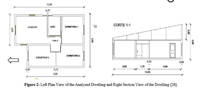
Figure 3 details the evolution of indoor temperatures on June 27^th, 28^th, and 29th. These three days were selected as they present the lowest outdoor temperatures of the autumn-winter period. On June 27^th, the room with the lowest temperature was the Dining Room at 9.1ºC, while the bedrooms ranged between 9.4ºC and 10.4ºC, when the minimum outdoor temperature reached 1.5ºC. On June 28th, the minimum outdoor temperature recorded was -3.4ºC, with the minimum bedroom temperatures ranging between 7.7ºC and 9.5ºC, and the Dining Room at 7.4ºC. Finally, on June29^th, the minimum temperatures were as follows: Dining Room 7.9ºC, Bedroom 1 9.8ºC, Bedroom 2 9.8ºC, Bedroom 3 8.0ºC, and the outdoor temperature at -2.8ºC. In Figure 4, the graph shows the indoor and outdoor temperatures for the west baseline case. The minimum outdoor temperatures are the same as for the south baseline case. On June 27^th, the minimum temperatures ranged from 9.4ºC to 9.7ºC for all rooms, while on June 28^th they ranged  from 7.7ºC for Bedroom 2 to 8.2ºC for Bedroom 1. Lastly, on June 29^th, the minimum temperatures were 8.0ºC for Bedroom 2 and 8.5ºC for the Dining Room

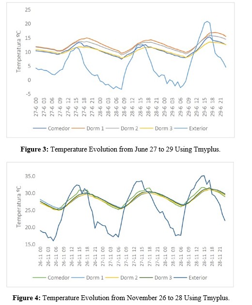
Figure 4 shows that the maximum temperature was 31.7ºC on November 28th, recorded in the Dining Room, followed by Bedroom 3 with 31.5ºC, while the outdoor temperature was around 35.1ºC. On the previous days (November 27^th and 28^th), the maximum temperatures in the bedrooms ranged between 29.6ºC and 30.5ºC. Table 9 details the average indoor temperatures and thermal amplitudes for June 27^th, 28^th, and 29^th. The average indoor temperatures ranged from 10.0ºC in Bedroom 3 to 13.2ºC in Bedroom 2. The thermal amplitudes in the bedrooms ranged from 2.4ºC in Bedroom 3 on June 27th to 7.0ºC in Bedroom 1 on June 29th. During the summer period, Bedroom 2 had the lowest average temperature at 27.4ºC with a thermal amplitude between 4.5ºC and 4.7ºC. Bedroom 3 had the highest indoor temperature at 29.1ºC and a thermal amplitude of 5ºC.

                                      Table 9: Average Temperatures of Interior Premises and Thermal Amplitudes.

We now analyze the heating load required in each room of the house depending on the orientation and the simulated day. For this purpose, Table 10 shows the daily total auxiliary energy values needed to maintain a temperature of 22.1ºC for the winter period and 24.4ºC for the summer period. The rooms named Toilet (house bathroom) and the Hallway were added because both contribute to energy demand. The total heating load of the house, with values of 56.4 KW (June 28), 62.1 KW (June 27), and 41.9 KW (June 29). Where Bedroom 1 was the room with the highest heating load demand on all three days. Ordering from highest to lowest total heating load of the house, the east orientation follows with a daily average of 58.6 KW, where Bedroom 3 was the room with the highest energy demand during the three days of tests. Analyzing Table 10 shows lower cooling demand values with an average of -54 KW. Bedroom 1 had the highest energy demand with an average of -11 W, followed by Bedroom 2 with -10.9 W and Bedroom 3 with -10.8 W.

Table 10: Heating and Cooling Thermal Load in Kw Required in Each of The Premises, to Maintain the Interior Temperature Between 22.1°C (Winter) And 24.4°C (Summer).

Conclusion

In this article, the Typical Meteorological Year (TMY) for the city of Salta has been generated using five sets of different weighting factors, previously unpublished. Such information is crucial for the accuracy of results in computational simulations of building energy performance, which is our ultimate goal. The results reflected that the chosen methods to design the Typical Meteorological Year resulted from the combination of the methods called TMY1, TMY2, and CHAN, this method was named TMYPlus. The TMY1 method was chosen for the selection of the TMM for the meteorological variable of dry bulb temperature, while the TMY2 method was selected for the TMMs of the meteorological variables of dew point temperature and wind speed. The total daily solar radiation on a horizontal plane was weighted according to the CHAN method. The combination of all these weighting factors forms TMYPlus. Along the way, computational codes have been developed for the implementation of the methodology followed to generate the TMY, allowing the results to be easily updated as new experimental data becomes available. Thanks to this study, Salta is now the third Argentine city with a TMY, after the Autonomous City of Buenos Aires and Santa Fe. The codes developed here are directly applicable to any other locality with a sufficiently complete set of meteorological data. It is our intention to apply them to the design of social housing produced by provincial governments, enabling more accurate modeling of the thermal behavior of buildings.

The simulation results applying TMYPlus showed that the South orientation is the best adapted to reducing energy consumption, both in winter and summer periods. The heating load of the house  for the winter period was 53.5 KW, with Bedroom 3 having the highest heating load during the three days of testing. The average cooling load in KW for the summer period was -54 KW. Bedroom 1 had the highest energy demand with an average of -11 W, followed by Bedroom 2 with -10.9 W and Bedroom 3 with -10.8 W. Based on the obtained data, it is strictly recommended to implement bioclimatic construction strategies in the simulated house. Thanks to the obtaining of TMYPlus and the application of energy efficiency strategies, up to a 30% energy saving in heating and cooling consumption can be achieved in this house.

References

- IEA. Energy system: buildings. International Energy Agency. (accessed 26 April 2024).
- Esteves, A., & Gelardi, D. (2006). Técnicas constructivas y materiales de bajo costo energético en la arquitectura sustentable. caso proyecto y construcción de vivienda en centro-oeste de argentina. Actas del XI Encontro Nacional de Tecnología no Ambiente Construido (ENTAC), 3629-3638.
- ASHRAE, Handbook Fundamentals, Chapter 24, (1989). American Society of Heating Refrigerating and Air- Conditioning Engineers.
- Hall, I. J., Prairie, R. R., Anderson, H. E., & Boes, E. C. (1978). Generation of a typical meteorological year (No. SAND-78- 1096C; CONF-780639-1). Sandia Labs., Albuquerque, NM (USA).
- IRAM 11605, (1996) "Aislamiento térmico de edificios, Condiciones de habitabilidad en viviendas". Institute de Racionalización Argentina de Materiales.
- Bre, F., & Fachinotti, V. D. (2015). Generación del año meteorológico típico para la ciudad de Santa Fe en la región litoral argentina.
- Bre, F., Fachinotti, V. D., & Bearzot, G. (2013). Simulación computacional para la mejora de la eficiencia energética en la climatización de viviendas. Mecánica Computacional, 32(37), 3107-3119.
- Roriz, M. (2012). Arquivos climáticos de municípios brasileiros. Relatório de pesquisa.
- Qingyuan, Z., Huang, J., & Siwei, L. (2002). Development of typical year weather data for Chinese locations. ASHRAE transactions, 108(Pt 2), 1-17.
- American Society of Heating, Refrigerating and Air- Conditioning Engineers (2009b). ASHRAE Handbook – Climate Design Data 2009.
- ASHRAE, Handbook Fundamentals, Chapter 24, (1989), American Society of Heating Refrigerating and Air- Conditioning Engineers.
- DOE-2, (1980). Reference Manual Part 2, Chapter VIII, National Technical Information Services, US Department of Commerce.
- Hui, C. M. (1996). Energy performance of air-conditioned buildings in Hong Kong (Doctoral dissertation, City University of Hong Kong).
- American Society of Heating, Refrigerating and Air- Conditioning Engineers (2009). ASHRAE Handbook-Fundamentals.
- Marion, W., & Urban, K. (1995). User's Manual for TMY2s (Typical Meteorological Years)-Derived from the 1961-1990 National Solar Radiation Data Base (No. NREL/TP-463- 7668). National Renewable Energy Lab.(NREL), Golden, CO (United States).
- ASHRAE, (2002). International Weather for Energy Calculations (IWEC Weather Files) User’s Manual, Version 1.1.
- Wilcox, S., & Marion, W. (2008). Users manual for tmy3 data sets (revised) (No. NREL/TP-581-43156). National Renewable Energy Lab.(NREL), Golden, CO (United States).
- Mandurino C., P. Vestrucci, (2009). Using meteorological data to model polluted and dispersion in the atmosphere, Environ. Model. Soft. 24 (2009) 270e278.
- Jiang, Y. (2010). Generation of typical meteorological year for different climates of China. Energy, 35(5), 1946-1953.
- Ohunakin, O. S., Adaramola, M. S., Oyewola, O. M., & Fagbenle, R. O. (2013). Generation of a typical meteorological year for north–east, Nigeria. Applied Energy, 112, 152-159.
- Rahman, I. A., & Dewsbury, J. (2007). Selection of typical weather data (test reference years) for Subang, Malaysia. Building and Environment, 42(10), 3636-3641.
- Chan, A. L. S. (2016). Generation of typical meteorological years using genetic algorithm for different energy systems. Renewable Energy, 90, 1-13.
- Yang, H., Li, Y., Lu, L., & Qi, R. (2011). First order multivariate Markov chain model for generating annual weather data for Hong Kong. Energy and Buildings, 43(9), 2371-2377.
- 26. Ruiz López, (2021). Tesis de grado Eficiencia energética de una doble fachada verde para tres climas de la provincia de salta. Universidad Nacional de Salta.
- Larsen, S. F., & Lesino, G. (2001). Modelo térmico del programa SIMEDIF de simulación de edificios. Energías Renovables y Medio Ambiente, 9, 15-24.