The Application of the Theory of Variable Speed of Light on the Universe

Introduction

In 1912, Vesto Slipher discovered a red-shift in the spectra of galaxies for the first time [1]. More and more, a systematic relationship between red-shift and distance became apparent with the successful determination of the distances of galaxies by Edwin Hubble, done from 1925 [2]. Based on this relationship, Georges Lemaître first presented in 1927 a dynamic world model with a well defined beginning [3].

Since that time, most of the physicists did not consider a stationary cosmos without temporal development to be a likely scenario. It was seen as a validation of Albert Einstein’s General Relativity Theory, which was difficult to be brought in line with a static universe, anyway. The red-shift was interpreted as escape velocity of the galaxies unanimously, even if Lemaître emphasized from the beginning that the galaxies are not moving away from each other but only “the space is expanding”. There were attempts to compensate the escape speed of the galaxies by creation of matter and to ensure a static universe in this way, but the vast majority of cosmologists committed themselves to the Big Bang model, whose exact properties continue to be the topic of perpetual research and discussions.

But even the Friedman-Lemaître solutions with cosmological constant Λ were not able to explain the basic properties of the universe coherently [4]. Today, the so called Cosmological Standard Model in form of the ΛCDM model includes in addition to that a phase of inflation, so called Dark Energy and Dark Matter, whose existence has not been proven so far. The number of necessary parameters has increased over time more and more and with the freely definable distribution of Dark Matter it has reached a quasi-unlimited amount, in which the observed flatness of the universe in the Standard Model, nonetheless, appears as an unexplained unbelievable coincidence.

It is the authors opinion, that there is something we do not understand correctly, if an extremely unlike coincidence is necessary for the theory to be valid. Indeed, it is the question, whether the Standard model fulfills the criteria of a good theory. It shall not be misunderstood: The Standard Model is the best theory we have. Still it is the time to challenge essential, generally accepted viewpoints in cosmology and to search for better ways.

In [5], a theory of variable speed of light was introduced, which is based on Special Relativity Theory and the equivalence principle, but it disregards the covariance principle. Not only is it a theory of variable velocity of light, but moreover, it is a theory of variable scales, because a consequent treatment of a variable speed of light enforces the variation of a series of additional scales. But one ends up at a closed and contradiction-free system.

Human beings tend to regard their own scales as absolute. And that is certainly true in many areas, not only in physics. As it was difficult for the human mind to accept the earth not being the center point of the universe, so, today, the postulate of the constancy of the speed of light is an expression of this literally egocentric mind set. All has to benchmark against our scale. Maybe slowly the time is about to come to clear this position, too. But up to now, rather it is firmly assumed that the entire universe is expanding, than it is only vaguely taken into consideration, that the length scale on the earth could become smaller. The main-stream believes, that a variable polarizability of the vacuum would not be compatible with the observations and, thus, is obsolete. The only one, however, with which it is not compatible, is this mindset.

A local measurement of the speed of light always results the constant value c0 without doubt. But to invoke this as proof of the speed of light being constant at all locations and every time is not correct. Because a local measurement would not notice any deviation, even if the speed of light should have changed. Einstein has introduced the constancy of the velocity of light, accordingly, as postulate at the beginning of his paper of 1905 [6].

With the assumption, that gravitation can be explained by a variable polarizability of vacuum, the classical tests of the General Theory of Relativity can be reproduced, which means all effects in weak fields. In strong gravitational fields, however, the differences between the theory of variable speed of light and General Relativity are of fundamental nature. Instead of refusing the theory of variable speed of light due to that, however, it should be regarded as a legitimate alternative for the description of gravitation

Robert Dickes Universe

In his paper from 1957 [7] Robert Dicke extended not only the approach of Harold Wilson [8] about the electromagnetic nature of gravitation, but he also designed a visionary picture of the cosmos, including some very bright ideas.

After he had outlined the concept of variable speed of light, he showed that the cosmic redshift does not necessarily have to represent an actual movement of the objects but can be reduced solely to a modification of length scales caused by the temporal variation of the gravitational potential in the universe without the galaxies executing an actual escape movement. He assumes a flat static space of homogeneous density.

According to Dicke the Big Bang is the fact, that the light started to spread in the beginning at the same time in the whole universe. The boundary of the universe is defined by the edge, from where light is reaching us. However, in Dickes approach the temporal development of the refractive index does not follow directly, but he makes additional arbitrary assumptions describing a temporal evolution.

Alexander Unzicker has enhanced this model and clarified especially the lapse of time for different positions of an observer [9].

According to the theory of variable speed of light in the version suggested by the author in [5], there is a fixed relationship between the potential of the universe, the propagation of light and the velocity of light. As will be outlined in the following, this leads to a universe, which exhibits qualitative main streaks of Dicke’s and Unzicker’s model.

The standard model is based on the Friedman-Lemaître-equations. The imagination of flyingaway galaxies, that are decelerated by their mutual attraction, is replaced by a model, in which the apparent movement and deceleration of the galaxies are replaced by a modification of the space-time itself.

Preconditions

To be able to come to a consistent world model, at first one has to be clear about the preconditions, which the model shall fulfill. They must, on the one hand, enable the representation of all properties of interest, on the other hand they should be as general and simple as possible. With this in mind, the following most simple assumptions are made:

• Gravitation can be described by a variable velocity of light.

• The cosmological principle is valid.

• The baryon density stays constant for a reference observer.

Standard Model. The first assumption does claim nothing less than the conjunction of gravitation and quantum physics being a prerequisite. It is not searched for in a second step, but we assume that gravitation is a secondary effect of the electromagnetic interaction between charged particles.

A curved space in the General Theory of Relativity means within our picture, that a light wave front propagates along curved paths caused by a gradient of the refractive index of vacuum according to Huygens’ law. To assume a gradient in the whole cosmos, though, violates the cosmological principle, which requests large-scale uniformity. Inasmuch point 2 in our model – the assumption of the cosmological principle – is equivalent to the requirement of a flat space. Therefore, a flat space is no extra demand but a strict consequence of the preconditions of the model. In the Standard Model, however, the flatness of space is a problem, because the measurements suggest a flat space, but the conditions for it have to be fulfilled extremely accurately without an explanation being offered by the Standard Model.

Dicke’s approach is able to explain the cosmological red-shift of the galaxies as an effect of the variation of the potential of the universe. This is expressed by the third request from above. A fictitious observer, whose potential remains constant, would not notice any movement, the density of matter in his universe would stay constant. The movement of the objects, hence, only appears as such.

Einstein and some other cosmologists even advocated the Strong Cosmological Principle stating, that there should not be a temporal variation of the cosmos. Due to the observations, the idea of a steady state universe is hardly supportable any more, but the assumption of a temporally constant matter density in the universe fulfills one aspect of the Strong Cosmological Principle at least to some extent.

Points of View

between spatially or temporally separated locations. In our recent paper, static potentials were examined and only spatial variations of the refractive index were discussed. In case of the universe, however, the interesting topic is about the temporal evolution of the universe as a whole. With the cosmological principle, we assume, that the large-scale matter distribution is homogeneous and we regard n = κ2 as constant in space throughout. Thus, it only remains to examine its temporal change. The present lends itself a reference point, at which n = 1. All quantities then are represented in relation to present-day values according to fixed rules, see [5], equations (7) – (21).

Essentially, there are two standpoints of an observer to be differentiated. The first observer, let it be called the reference observer, shall be positioned at a stable reference potential of today and he shall remain on this potential for all times. He describes the universe of the past and the future in relation to this reference with a uniformly running clock with time t. Today, the age of the universe is tu . The baryon density stays constant for the reference observer, because his length scale does not change with the potential of the universe. Even if this virtual observer does not exist in the universe, because the background potential of the universe is decreasing steadily, it is rather helpful. The space scale of the reference observer corresponds to the “comoving distance” in the Standard Model.

The second standpoint is consequently local and it is related always to the local time and the corresponding potential. The proper time τ represents the “age” of an object.

A today’s astronomer, who analyzes light information arriving at us now, essentially takes the standpoint of the local observer.

Space and Time

To get a correct picture of the universe, first of all, we have to think about, which “distance” is significant for the gravitational interaction at all. It became clear, as soon as we treated a variable index of refraction, that the usual distance in meters is no well defined quantity any more, but depends on the refractive index. Spatial and temporal variations can play a role.

We look at a laboratory, in which the polarizability is ε0 initially. It shall be assembled an experiment in the laboratory, that measures the electrical force F between two charges q1 and q2. The distance between the charges shall be r.

Now we consider what happens, if the index of refraction varies. Herein, we distinguish between the views of the reference observer and the local observer, which tries to get a consistent picture of the situation only taking into account locally measured quantities. The distance definition of reference and local observer are identical in the initial stateNow the index of refraction shall be increased by the factor n = k². The reference observer now finds" D  The distance between the charges r shall remain unchanged and their location is not varied.

The force, therefore, decreases by the factor κ². If the same situation is to be described by the local observer, he notices the measured values in a different way. For the local observer, the refractive index is always equal to 1, thus, the permittivity of vacuum is ε = ε0, but the distance seems to be increased to r0 = rκ. For the local measured force it means:

So both observers come to the same result of the force, though, having a different perception of the structure of the experiment now.

One can ask, why the electrical force between two charges is diminished at all, if “space” is between them. If there is some attenuation already and one doubles the distance, then the force is diminished to a quarter. This is described by Gauss’ law adequately. If the index of refraction ε is increased, it results in a stronger attenuation as well. It can be imagined in a way, that the medium within the space can be polarized. The vacuum is filled with orientated dipoles. These dipoles generate a compensation field attenuating the primary field of the two charges more and more with increasing distance.

Both situations can be regarded as equivalent. It only depends on the “amount” of dipoles located between q1 and q2. Herein, both observers agree. But whether the resulting force is counted among the polarizability of the vacuum or among a certain distance, is a pure matter of definition. Space (and time) per se are not defined firmly in a Newtonian sense but only relatively. Each observer can set the index of refraction κ = 1 and, hence, himself as reference.

If it is respected that clocks run slower by the factor κ for the local observer, the distance measurement by means of the light travel time works as well: the local observer measures the distance r₀ by measuring the (proper)  time the light needs to cross it.

The reference and the local observer, therefore, come to self-consistent measurements of space and time, but having a different interpretation. Because the reference observer is only an arbitrary choice as well, every observer is of equal value and can define his view point as reference.

On the ground of a variably polarizable medium, therefore, the structure of a Newtonian space-time can be established. We stay at the assumption, that gravitation as electromagnetic phenomenon has analog properties as the electrical force itself. For Newton, the absolute space and the absolute time were simply given, because the physical measurements at that time gave no reason to have concerns about it. In General Theory of Relativity, the matter-free space is equal to Newton’s space as well. Matter only “bends” it a little bit. The theory of variable speed of light drops Newton’s absolute space completely and defines the empty space as well as only relative.

Now we go a further step ahead and try to describe interactions, if the polarizability of the vacuum varies with time. The variation shall happen in the entire space simultaneously, the polarizability, therefore, shall be spatially constant at all times. For that, we further assume, that all distances stay the same for the reference observer. As a picture, we imagine an electrical charge (transmitter), which sends a spherical wave of photons into the space. Because the polarizability is always spatially constant, the spherical symmetry of the wave field is preserved at all times, even if the refractive index of the vacuum and, therefore, the propagation velocity of the light is modified. Because in case of a temporal change it does it simultaneously in entire space. If a spherical wave hits the observer(receiver), several things are of relevance.

The observer interprets the incoming spherical wave straightly locally. It is irrelevant for the shape of the incoming wave front where on the way the speed of light has changed. The light travel time being a suitable length scale in a constant medium is not a reliable quantity for the estimation of the strength of the interaction any more.

If the reference observer is on the same gravitational potential as the receiver    then their length scales match. Hence, a distance measurement to the sender is also the reference distance.

If the index of refraction of the sender T at the time of emission is different to that of the receiver at the reception, a red-shift occurs at the receiver. In the case of our universe the speed of light in the past was greater than today 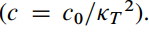  Light was emitted with higher frequency and larger wave length. The wave length did not vary during the propagation, but the frequency has slowed down at the arrival today by the factor HT ². Hence, it reaches us red-shifted by the factor H_T , because the potential of the universe experiences a temporal change, but being spacially flat all the time [7,5]. We assume that gravitation is an electromagnetic interaction of its nature. And just as the distance is adjusted by the red-shift in case of the “luminosity distance”, we also assume, that the red-shift of a distant galaxy attenuates the gravitational force. In the Standard Model, the luminosity distance is defined by the “comoving distance” d_C :

in the case of a flat space. The “comoving distance” is defined in the Standard Model in a way, that it represents a constant distance scale despite the expansion of the universe. Hence, it is equivalent to the reference distance r in the theory of variable speed of light. The luminosity has the unit W/m2 as a flux of energy and decreases quadratically with increasing distance, because the visible cross section is relevant in case of the emission of radiation. The incoming power of radiation is reduced quadratically, too, if the observed light of a galaxy is red-shifted, because less photons are arriving per unit of time and, additionally, those photons have less energy.

Herewith we state the hypothesis, that the luminosity distance is the length scale, which is significant for the strength of the electrical and the gravitational interaction as well.

With 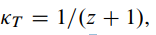the red-shift factor is identical with the scale factor a in the Standard Model. The distance significant for the strength of the interaction, therefore, is:

The definition of the distance introduced here is not a new arbitrary ingredient to the theory. It follows solely from the laws of Special Theory of Relativity. As carved out in [5], the rest energy of an unmoved body is responsible for the gravitational force. The rest energy of a test body is decreased at a location with deeper potential and, hence, the gravitational force is reduced compared to Newton’s law. In case of the universe, we regard the matter as unmoved as well. Only the potential becomes deeper over time. The red-shift effected by that leads to a likewise reduced rest energy from the view of the observer. Both situations are equivalent in the frame of the theory of variable speed of light.

It is interesting also to imagine, what happens, if the speed of light decreases at the location of the receiver. Because the length scale is decreased as well, the receiver cuts out a smaller area of the spherical wave by the factorHR^2. The strength of the interaction is attenuated by the factor(H_T /H_R)². For the local observer it means also, that the transmitter now has a red-shift of H^T /H^R and immediately possesses a greater distance by the factor of H^R This is a completely local phenomenon and there is no time delay related with the speed of light. The red-shift can turn out to indicate a “superluminal velocity” without problems, if it is interpreted as velocity.

Einstein’s solution was to define a curved space-time, in which the speed of light is constant. He was able to find a consistent formulation with the Equivalence Principle and the Covariance Principle, which described the gravitational phenomena in the solar system correctly.

The theory of variable speed of light chooses a similar way. The observations are described within an principally flat space-time, but the curved light-paths are taken into account with a variable velocity of light.

The Potential of the Universe

The basic idea from [5] is, that the relative change of the potential of the universe is equal to a relative change of the refractive index of the vacuum:

With that, the scale factor a or the velocity of light, respectively, is connected unambiguously with the potential of the universe. If we know the potential of the universe and its development over time, we are able to deduce the development of the scale factor.

We regard the universe as sphere of uniform density according to the Cosmologic Principle. We are located at its center point. Now we calculate the Newtonian potential of this sphere by integrating the contributions to the potential across the entire volume. We assume the luminosity distance 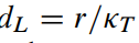according to equation (6) to be the effective distance.H_T (r) is the red-shift of the “transmitter”, as we measure it today. Thereby, we evaluate the situation from the view of the reference observer, which takes the present potential of the universe as a permanent point of reference.

The infinitesimal mass element 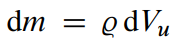with constant density g and volume element dVu produces the potential in the center point of a sphere

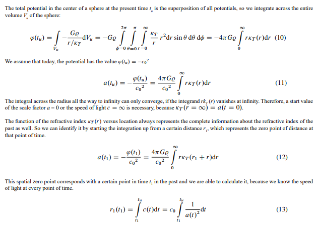
At this point it makes sense to describe the sequence of time not by the time of the reference observer t, but to change to the proper time τ of the local observer. All age indications in the universe are based on the observation of processes and these processes happen in proper time. The calculation in reference time does not have any advantage here. Nevertheless, it is important to be conscious about this relation all the time. If one wants to describe the lapse of time in proper time τ, one has to convert the different clock speeds. The clock of the local observer runs slower by the factor a than that of the reference observer. Thus, (local) clocks ran faster in the past (a < 1) in relation to now.

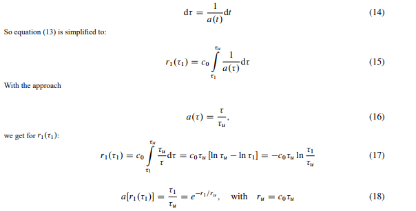
τ_u is the proper time elapsed since the beginning, thus, the age of the universe. The characteristic radius ru is the radius, which the visible universe would have, if light would have propagated with constant speed from the beginning, referred to as the Hubble-radius in the Standard Model. In the model of variable speed of light, the age of the universe τu is identical with the Hubble-time. The scale factor a (τ) at a point of time in the past corresponds to a red-shift H_T [r(τ)] from a certain distance, from where light arrives at us today. If the scale factor is the linear function a(τ) D τ/τu, then the red-shift of a distant galaxy is:

This relation of the scale factor we insert now into equation (12).

Due to the properties of the e-function it is possible to pull a factor with constant distance in front of the integral. The relation is valid for all times τ and the index can be omitted, because the point of time τ1 can be chosen freely. With that, the scale factor is composed of the today’s value and the red-shift of the past.

This solution is valid for all times. But this merely means: If the red-shift in relation to the distance represents an exponential function at a specific point in time, then it is an e-function at all times. And there is an extrapolation into the future for any arbitrary configuration HT (r). What does this all mean? We assume, that at the beginning, the polarizability of the vacuum was zero, which means that the speed of light was infinitely large. As soon as light started to propagate, however, matter began to interact mutually, which decreased the speed of light and slowed down the initially very rapid propagation. As a consequence, the rate of decrease gradually slowed down. In sum it is a stable process, at which the polarizability of the vacuum steadily increases and the rate of increase is slowing down.

A numerical simulation shows, that any initial configuration is washed out incrementally and the spatial function of the red-shift results eventually in the solution HT (r) e—r/ru . The temporal evolution of a(τ) increases monotonously at any point in time. In opposite to the Standard Model, it is robust against the initial conditions and anything like a “collapse” is mathematically excluded. It is possible now to calculate the integral to determine the present-day potential in equation (10). It, too, converges with an infinite radius.

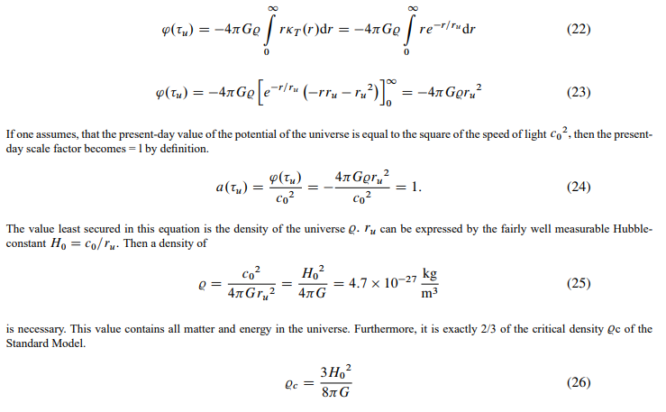
Robert Dicke had in his model a cosmos in mind [7], in which distances are assigned conventionally without weighting with the red-shift. The red-shift of the galaxies he was able to explain by the steadily decreasing potential of the universe. This increase of the absolute value is caused by a growth of the radius of the visible universe in his model. For the above mentioned reasons we do not regard this appraisal of distances in the universe as sustainable. Nonetheless, this idea is groundbreaking, because the variable potential of the universe acts directly onto the space itself and not onto the motion of the galaxies like in the Standard Model. This is a totally different mechanism and, in the eyes of the author, the correct way for a deeper understanding of the cosmos.

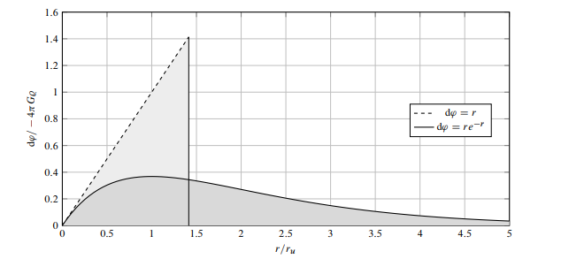
Figure 1: The values which each spherical shell of radius r contributes to the potential of the universe. The total potential φ(tu) is equal to the area below the curve. Dashed line: Rigid sphere with finite radius, solid line: universe of the variable speed of light

The contributions to the potential at small radius r agree at the beginning to those of an equally dense, unmoved sphere like in Robert Dicke’s model, shown as dashed line in figure 1. Its contributions to the potential increase linearly, because the impact onto the potential in the center of the sphere decreases with 1 / r, but the area of the spherical shells increase with r₂. They diverge for infinite radius, the integral over them even more so.

In the universe of variable speed of light, their impact declines with increasing distance r due to their rating with the red-shift factor K_T . The integral across all contributions is finite, too. An unmoved sphere with radius p²ru would have the same potential as the universe, because:

Temporal Development of the Cosmic Potential

To calculate the potential at an arbitrary moment, the index of refraction of the observer a(τ) D a(τu)K_T (r(τ)) has to be respected

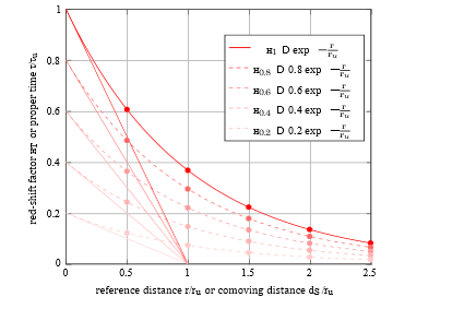
Figure 2: The refractive index K_T as a function of the reference distance r. The weaker curves are Hubble diagrams of the past from the view of the reference observer (today K_R 1)K0.8 meansK_R 0.8 and also τ 0.8 τu. The dots represent galaxies. They change their red-shift with time, but remain at the same distance r.

The present-day Hubble diagram K₁ in figure 2 is a look into the past. At any distance r one can read the index of refraction K_R(τ) a(τ) of that time and, thus, the speed of light. The curves of the past represent a vertical compression of the contemporary Hubble diagram and a horizontal shift as well. The speed of light was higher in the past (less slope means more distance per time). The Hubble diagram of the past starts, therefore, at the dedicated smaller K_R-value. For the reference observer, the galaxies preserve their distance r. The characteristic radius (Hubble-radius) of the universe ru is temporally invariable (from the view of the reference observer). In the Standard Model also the expansion of the space has to be regarded for the “true” expansion of the cosmos (particle horizon).

If somebody puts oneself in the place of a local observer, then the temporal development of the universe appears other than to the reference observer.

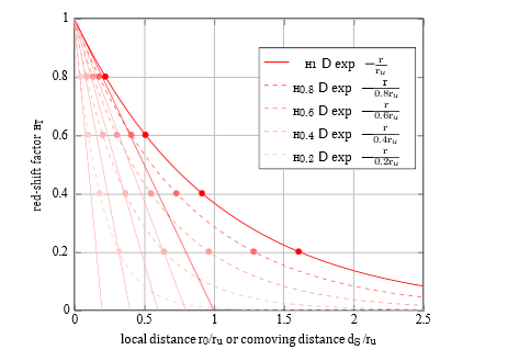
Figure 3: The refractive indexH_T as a function of the local measured distance r0. The weaker curves are Hubble diagrams of the past from the view of the local observer (alwaysHR D l). H0.8 means the curveH(r0) at the proper time τ D 0.8 . τu.

A local observer like in figure 3 naturally puts his potential as reference and, hence, a(τ) l at all times. The distances of the galaxies apparently are growing, because the length scale is decreasing appropriately. The local measured characteristic radius of the universe ru0 is increasing, too. The red-shift of the galaxies does not change relatively tohe particular local observer. Hubble diagrams from the past seem to be compressed in x-direction.

The universe exhibits a high self-similarity. Nonetheless, there is a starting point, which reason can not be given. The question, which was before, remains as groundless as in the Big-Bang model.

The term “Big-Bang” does not fit very well any more. “Primordial Flash” meets the matter significantly better in terms of the theory of variable speed of light as an electromagnetic theory.

The value of the density g of matter and energy, respectively, drops out, because all relations are defined as relative quantities. Indeed it depends on a reference observer, which defines his scales as reference being a local observer at the present time.

Let us assume matter density being greater by a factor of 8 today. The scale factor would be set to 1, nonetheless. However, clocks would have run slower by a factor of 2 from the beginning and and would indicate only half of the age of the universe. One would have to wait double the time, then we would arrive at today’s age of the universe again and the density of the universe would have decreased to the contemporary value. In other words: the initial density is not a value at all, that can be defined. The only question is, how much proper time since the primordial flash has passed. This can be defined in units of atomic frequencies doubtlessly.

There is no initial condition in form of an absolute “density of the universe”. It has to be “something” only and it has to be distributed uniformly to some extent. An astonishing result: A different matter/energy density of the universe would change length scale and lapse of time in a way, that the universe would look exactly the same. Quite contrary to the Standard Model, in which the present shape of the universe demands the compliance of the initial conditions in highest precision. Additionally that means, that constants of nature, which we regard as fundamental – as the velocity of light c0 and the field constants ε0 and μ0 – are variable from the view of a reference observer and that the values differ indeed dependent on location and time. Measurements executed by a local observer always result in the same values, though. These quantities, therefore, are variable as well as constants of nature according to the particular point of view.

Olbert’s paradox has to be augmented by an additional facet. Olbert argued a static infinite uniform cosmos would be infinitely bright. The present solution of this problem consists of the argument, that light only arrives from a finite space area at us, even the universe may be infinite itself. According to our theory of variable speed of light this is not valid any more. We can see light from the entire infinite cosmos. However, light from large distance is red-shifted to such an extent, that the total arriving light energy, nevertheless, is finite.

Another interesting issue is the development of the matter/energy density in the universe. It is essentially linked with the baryon density at least as of a certain point of time. For the reference observer, the baryon density gb, thus, the number of baryons N per volume V according to our basic assumptions is constant at all times:

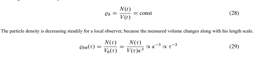
The particle/energy density at the beginning was infinitely large for the local observer. Because the mass/rest energy of the elementaryparticles results in the same values all the time, the mass/energy density goes along with the particle density.

The primordial state is characterized by an enormous instability. The evenly distributed matter contains a high potential energy, which is released as gravitational energy at agglomeration and largely is converted into kinetic energy. That represents the motor for all occurring processes in the universe and is the source for any structure formation.

Thus, the scenario of the genesis of the universe is essentially the same in the standard model as well as in the theory of variable speed of light. But there can arise great differences in the individual stadia like nucleon synthesis or building or the formation of the galaxies.

The local observer will interpret the red-shift as escape velocity at first glance, the distances to the galaxies seem to increase indeed as well. The reference observer, however, would describe the situation such, that the gravitational/electromagnetic interaction in the beginning had an extremely large range. Thus, the state, which is described here, does have by all means some similarity with the Big Bang in the Standard Model, but it differs in several fundamental aspects, nonetheless.

The Interpretation of the Hubble Diagram

In the recent years, the range of the Hubble diagram was extended up to a red-shift of z > 2 by the observation of more than thousand supernovae of type Ia and its precision has been improved significantly.

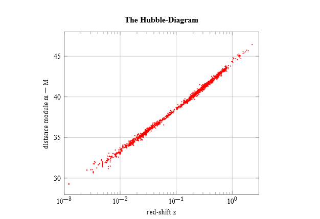
Figure 4: The distance module m − M as a function of the red-shift z                                                                                                             

Figure 4 :shows the distance module, essentially the distance, as a function of the red-shift of 1700 supernovae type Ia from the Pantheon+ data set [10]. In the Standard Model, very specific details about the expansion of the cosmos, vacuum energy and dark matter are deduced. For the sake of simplicity, all absolute brightnesses M were assumed here to be -19.5 mag, because the model itself influences the exact determination of M.

The theory of variable speed of light opens here a very different perspective. When following its line of arguments, the Hubble diagram has to be looked at from a very different angle. As Robert Dicke showed, the red-shift of galaxies can be explained by an increase of the polarizability of the vacuum since the primordial beginning. In an imaginary reference space, in which the gravitational potential remains constant, the galaxies keep their cosmic position. The “flatness problem” does not exist here at all in the first place.

The reference observer perceives, though, that the length scale of a local observer keeps shrinking steadily, because his potential continues to decline. Because of that, the galaxies seem to be escaping from the perspective of the local observer. The gravitational potential was zero at the primordial moment, the local scale, thus, infinite, and the matter density infinitely large.

We can see from the equation of the luminosity distance (5), that the reference distance r (or the comoving distance, respectively) of a galaxy is contained here:

By dividing the luminosity distance dL by the red-shift z C 1 D 1H_T , we directly get the reference distance r of such a supernova. We plotH_T vs. the reference distance r and get a somehow modified Hubble diagram.

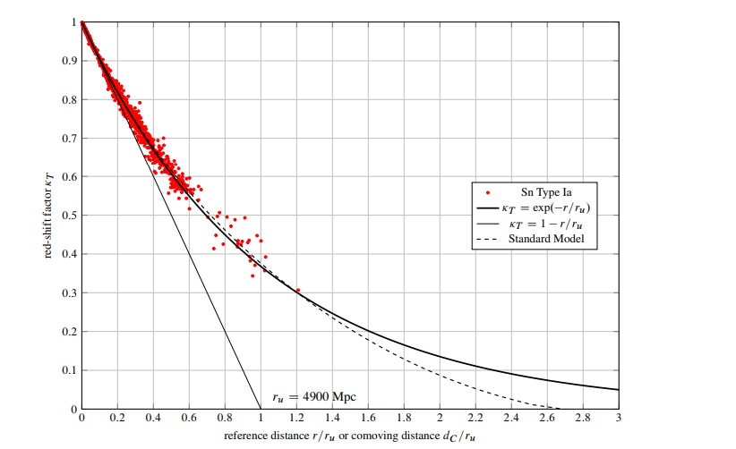
Figure 5: The Hubble diagram represented by the red-shift factor H_T as a function of the reference distance r or the comoving distance d_S , respectively. Near supernovae are tightly compressed in the upper left corner of the graph, the representation of the trend at high red-shifts is very sensitive in return.

The red-shift of the supernovae follows very well the above postulated trend of the exponential function. There is only the one parameter ru. Its value is around 4900Mpc according to the supernovae data. The red-shift factor HT in figure 5 drops with increasing reference distance r of the supernovae. Herein,H_T represents the scale factor a at the time of emission of the light, too. The data set ends at aboutH_T = 0:3, which corresponds to a reference distance of about 6000Mpc.

The value H_T = 0 is reached not until an infinite reference distance. At this point, the “horizon problem”, which is quite a problem for the Standard Model, is resolved. There is no horizon.

In the Standard Model, the graph cuts the x-axis, because light reaches us only from a finite distance. The cutting point corresponds to the “particulate horizon”.

The universe seems to have a finite radius Ru0 for a local observer, anyway. He assumes the speed of light being constant c0 all the time. The local observer recognizes the initial space, which the light has crossed with very high velocity, as strongly compressed with increased matter density.

The age of the universe is: 

The Hubble-constant H0 is connected tightly with ru , too. It is the slope of the function H_T (r/ at r 0.

The value of the age of the universe deviates somewhat from the accepted value of 13.8 billion years, and the value of Hubble’s constant lies outside the range of secured values of about 67 – 75 km/s=Mpc. But this shall not trouble us for the moment, because up to now, our considerations and calculations are about the rough shape of the universe, in first place. The discrepancies might be caused by the density fluctuations in our cosmic neighborhood. We live in a space area with considerably lower matter density [11], so deviations from our simple model are to be expected, since it is based on the assumption of uniform matter density.

Apart from that, there is only one unique free parameter in this simple form of the model. It is not fitted with several parameters in order to match as well as possible to the progression of the Hubble diagram as it is done in the Standard Model. Instead, it has to turn out, that the theory is able to reproduce the observations even with this one parameter. The deviations from this simple version of the model are not arbitrary and they must be extracted from the real distribution of matter.

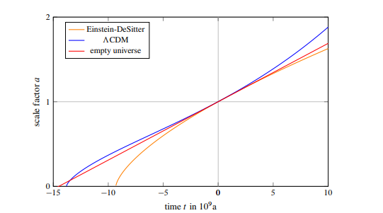
Figure 6: The scale factor of the Standard Model has approximately the same development as the so called “empty universe”, which corresponds to the model of the variable speed of light

As soon as one became aware of the astounding flatness of the universe, at first the EinsteinDeSitter cosmos was favored, which got along without the cosmological constant Λ yet, until it became clear, that the model could not be brought into agreement with the age of the universe. Particularly the precise survey of the supernovae type Ia convinced the community of cosmologists, that a nonzero Λ would bring the development of the scale factor closer to reality. Obviously, the trend of a in the Standard Model nestles more and more up against the linear function of the “empty universe”. However, the standard cosmology does not get around the unpleasant property of an infinitely steep slope at the beginning caused by the basic assumptions of the theory. This, in turn, increases the problems of structure formation to an unsolvable dilemma.

Problems of the Standard Model

The Friedman equations consider the kinetic and the potential energy of the matter in the universe. Herein, it is stated, that the galaxies do not move on the cosmic scale on the one hand, already emphasized by George Lemaître. The space expansion would be the reason for this seeming movement. But then it is argued on the other hand, that the galaxies attract themselves mutually and decelerate the escape velocity. Though, this deceleration strictly speaking is treated as a change in peculiar motion again, but then interpreted as variation of the expansion of space. Thus, a peculiar velocity is the reason for space expansion or its variation, respectively.

This is an illegal reinterpretation and, hence, a clear contradiction within the standard theory in the authors opinion.

No, in a flat, infinite space the gravitational forces onto galaxies cancel each other. Therefore, galaxies are not accelerated towards each other, the universe does not expand or collapse in the sense of a motion. Rather, the potential of the universe is varying and, thus, the scales, which depend on the potential. So, the potential acts onto the space itself without influencing directly the cosmological movement of the galaxies. Length scales are shortened over time, therefore, the galaxies appear to depart.

The presented model of the universe corresponds to the “empty universe” of the standard model. This is compatible with the observations, but it was excluded, because it did not appear meaningful in the frame of the Standard Model.

The Standard Model did not find a consistent representation of variable scales, which are, though, implicitly contained in it as well. A shrinking length scale instead of an expansion of space represents an immediately plausible explanation of the seeming expansion of the cosmos. However, this obvious explanation is strictly eschewed, because a variable length scale directly imposes a variable speed of light. And the constancy of the speed of light is a basic premise of the Standard Model.

As a consequence, a number of fundamental problems arise. The flatness problem was mentioned already. Another one is the horizon problem. When, according to the standard model, about 380000 years after the Big Bang the temperature had decreased far enough, such that the hot plasma converted into a gas of neutral atoms, the universe became transparent and light rays started to propagate for the most part in a rectilinear fashion through space. The oldest visible remains of the universe date from that point in time and constitute the so called microwave background. Due to the expansion of the universe, space areas were separated so quickly, that they did not interact to this day. This applies to all areas of the microwave background, which are separated by more than 1° in today’s viewing angle. Despite of that, a great homogeneity can be observed over the whole angular range. The hypothesis of Cosmic Inflation shall now explain, how these space areas could have exchanged information in order to establish thermal equilibrium.

The steep rise of the scale factor starting from the Big Bang causes the problems of structure formation. The extremely large speed of expansion in these early times would have prevented an agglomeration of matter to stars and galaxies. Only with the help of hypothetical Dark Matter, a structure formation can be described in the Standard Model.

In the theory of variable speed of light here presented, the scale factor is a linear function of time right from the beginning. Therefore, the mutual gravitational forces decrease much later and the much slower expansion right from the start does not foil the initial fluctuations like in the Standard Model. Thus, the structure formation could occur early and very quickly.

Unlike in the Standard Model, the entire universe is in contact since the beginning. There is no mechanism being able to separate it again. The horizon problem does not exist. Andreas Albrecht and João Magueijo show in [12], how the hypothetical assumption of a variable speed of light could solve essential problems.

Despite the excellent numerical agreements with observational data in many areas, the Standard Model has the shortcoming, that it operates with many additional ad-hoc assumptions and parameters. In other words: The Standard Model is full of epicycles, so that in the end, it runs into the problem of nonfalsifiability. The model, with its multitude of parameters, can (and has to) be adapted simply to any new observation. With that, the theory is degenerated to a pure describing model and, thus, has lost its capability of prediction.

The search after the Dark Matter more and more turns out to be like the unavailing quest for the ether more than a hundred years ago. This was given up not until Albert Einstein made the necessity of an ether as carrier medium of light obsolete with his Special Theory of Relativity [6]. Dark Matter is neither necessary nor possible in the theory of variable speed of light.

The situation even resembles the transition from the geocentric to the heliocentric world model. Of course, one can describe the planetary system as representation of the universe at that time from the viewpoint of the earth observer in its center. It is only a little bit cumbersome, the physical conceptions are not really consistent and a multitude of parameters is necessary to hold the loosely tied overall model together. The heliocentric world model of Kopernikus did not provide a real simplification, as long as it clung to circular orbits including epicycles. Only Kepler’s ellipses led to a fundamental simplification of the description of the planet’s trajectories. With Newton’s law of gravitation, the orbits finally could be explained by a single physical law and even the deviations of Kepler’s ellipses could be modeled as orbital distortion with the same law.

And of course, the universe can be described as in the Standard Model with the premise, that our local scales – the speed of light as a representative quantity – are the same in the whole cosmos. This requirement imposes itself on us, because all local measurements result the same values. But this essentially is a very geocentric point of view. In any case, a model with constant scales leads to just that Standard Model, which measures up already with the geocentric world model in terms of the number of needed parameters. And in a similar manner, the Standard Model is incapable of establishing a simple and closed structure, but it has to integrate new observations with ever new additional assumptions into the model instead of being verified and confirmed by new data. The James-Webb-telescope delivers the next textbook example of this through the observation of high red-shift galaxies, whose development is much too far advanced according to the Standard Model [13].

Conclusion

The theory of variable speed of light in the version outlined here is able to describe the basic structure of the universe according to the observations. The starting point is Robert Dicke’s insight, that the red-shift of the galaxies can be explained by the steady decreasing of the gravitational potential of the universe. The imagination of an “expanding space” is replaced by the equivalent concept of variable scales. Not the space as such is expanding, but the length scale is shrinking.

The temporal evolution of the scale factor is deduced from the theory with the help of only one single free parameter. The evolution is linear from the beginning and compatible with the observations. Thereby, many fundamental difficulties of the Standard Model dissolve, like Dark Matter, Dark Energy, the flatness problem and the horizon problem. The structure formation, too, is explainable much more easily by a linear evolution of the scale factor.

Acknowledgement

I am very glad having encouraging support by many colleagues and friends, especially Michael Wichmann, Christoph Parzinger, Verena Eckardt and Bernhard Schönlinner, Jakob Schönlinner, Alexander Unzicker, Dieter Seibold and John Miller. Thanks a lot for many fruitful discussions, valuable hints and error corrections, and also technical assistance.

References

1. Slipher, V. M. (1915). Spectrographic observations of nebulae. Popular Astronomy, Vol. 23, p. 21-24, 23, 21-24.
2. Hubble, E. (1929). A relation between distance and radial velocity among extra-galactic nebulae. Proceedings of the national academy of sciences, 15(3), 168-173.
3. Lemaître, G. (1927). A homogeneous universe of constant mass and increasing radius accounting for the radial velocity of extragalactic nebulae. Annales de la Société Scientifique de Bruxelles, A47, p. 49-59, 47, 49-59.
4. Friedman, A. (1922). Über die krümmung des raumes. Zeitschrift für Physik, 10(1), 377-386.
5. Schönlinner, M. (2026). “Gravitation as a Secondary Effect of Electromagnetic Interaction”. In: J. of Mod Phy & Quant Neuroscience 2(2), 1–19.
6. Einstein, A. (1905). “On the electrodynamics of moving bodies”. In: Annals of Physics (1905), pp. 891–921.
7. Dicke, R. H. (1957). Gravitation without a principle of equivalence. Reviews of Modern Physics, 29(3), 363.
8. Wilson, H. A. (1921). An electromagnetic theory of gravitation. Physical Review, 17(1), 54.
9. Unzicker, A. (2008). “A Look at the Abandoned Contributions to Cosmology of Dirac, Sciama and Dicke”. In: arXiv:0708.3518v5.
10. Scolnic, D., Brout, D., Carr, A., Riess, A. G., Davis, T. M., Dwomoh, A., & Zheng, W. (2022). The Pantheon+ analysis: the full data set and light-curve release. The Astrophysical Journal, 938(2), 113.
11. Keenan, R. C., Barger, A. J., & Cowie, L. L. (2013). Evidence for aâ?» 300 megaparsec scale under-density in the local galaxy distribution. The Astrophysical Journal, 775(1), 62.
12. Albrecht, A., & Magueijo, J. (1999). Time varying speed of light as a solution to cosmological puzzles. Physical Review D, 59(4), 043516.
13. Robertson, B. (2022). “Identification and properties of intense star-forming galaxies at redshifts z>10”. In: arXiv:2212.04480.