

Journal of Applied Surface Science(JASS)
ISSN: 2993-5326 | DOI: 10.33140/JASS


Research Article - (2026) Volume 4, Issue 3
Simulation of the Moiré Effect in a Volumetric Cube. Part I: Face View

Received Date: Sep 16, 2026 / Accepted Date: Oct 22, 2026 / Published Date: Nov 05, 2026
Copyright: ©2026 Vladimir Saveljev. This is an open-access article distributed under the terms of the Creative Commons Attribution License, which permits unrestricted use, distribution, and reproduction in any medium, provided the original author and source are credited.
Citation: Saveljev, V. (2026). Simulation of the Moiré Effect in a Volumetric Cube. Part I: Face View. J Applied Surf Sci, 4(3), 01-16.
Abstract
In a multilayered 3D display (volumetric cube), the moiré effect creates visual corridors. These corridors are characterized by angles whose tangents are rational numbers; they connect "focus" points located on the axes. The study presents a detailed analysis of the face (front) view. The authors calibrated the view in arctangent units and derived formulas to determine the focus points and corridor parameters. Computer simulation, combined with Radon and Hough transforms, confirmed the corridors’ characteristic inclination angles. The authors explained how the corridors traverse the volume, analyzed the influence of geometric parameters, and formulated the conditions for the moiré patterns in a cubic lattice. The results may be applied in crystallography and in developing methods to minimize the moiré effect in volumetric LED 3D displays.
Keywords
Moire´Effect, Volumetric 3D Structure, Rational Tangents, 3D Moire´, Volumetric Moire´,LED-Based Volumetric 3D Displays
Introduction
The moiré effect is an optical interaction between layers of periodic structure (grids, lattices) viewed in transmission. Moiré fringes are alternating dark and light regions. The effect is primarily considered in two dimensions, typically in coplanar layers [1,2]. Relatively rare, the moiré effect is studied in three dimensions, for example, on a plane plus a curved surface, in structures separated by a gap, in three-dimensional (3D) objects such as a rectangular parallelepiped (rectangular prism), wedge (triangular prism), and cylinder, as well as in measurements of 3D objects [3-14]. The moiré effect in essentially 3D structures was considered in [15,16].
In this work, we investigated a substantially 3D volumetric structure — a simple cubic lattice, which can alternatively be considered as a set of identical parallel untwisted layers in space; see Figure 1. Recently, the moiré effect in a cube was investigated [17]. Here, we present more detailed research, including multiple simulations and formulas.

Figure 1: Layers of the Volumetric Cube and the Local Camera System
In the face (front) view, the local camera axis z’(“main” longitudinal axis) is directed along the crystallographic direction with the Miller indices [100], which is perpendicular to the crystallographic plane (010); see References [18-20]. In such a layout, the Euler angles (α, β, γ) are (0, 0, 0); see Refs. [21,22]. We call it a face view [17]. Figure 2(a) shows the face view of the voxel cube, with the cube contours drawn over the simulated view image. However, these contours are ambiguous; for clarity, Figure 2(b) shows a sketch view from a slightly deviated direction.
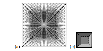
Figure 2: (a) Face View of the Volumetric Cube, (b) Schematic Sketch from a Slightly Deviated Perspective
An image with moiré patterns, see, e.g., Figure 2(a), is not uniform. The visual interference of multiple layers in a regular volumetric lattice manifests itself as "empty" and “filled” areas. One can recognize multiple horizontal, vertical, or slanted “alternating dark and light areas” (cited by Ref. [1]). These areas comprise “corridors” with reduced voxel density [17].
Based on the definition of the moiré effect given in [4], we associate these corridors with moiré patterns. Moiré corridors can be seen in a cubic lattice, in 3D displays, and in LED cubes [23-29].
This moiré effect in the volumetric cube is essentially multilayered [17]. It depends on the number of layers and appears only when n >5. see Ref. [20].
We sometimes increased or decreased the number of voxels in the cube, but the minimum thickness was 4 voxels (otherwise the corridors would not be displayed) [17]. We also investigated the the influence of distance and size.
In a volumetric display, moiré corridors distract the observer's attention from the useful 3D structure. Therefore, we should reduce, and ideally eliminate, this undesirable effect in volumetric 3D displays [30,31].
Materials and Methods
In our research, we position the global axes as shown in Figure 3.

Figure 3: Global Axes
To simulate the visual effect of the 3D structure from a finite distance, we used the Java version of Web VPython [32].
Number of Layers
Surprisingly, the corridors do not disappear at large values of layers. Fewer layers mean less detail; however, the corridors permeate the entire cube regardless of the number of layers (even when it is large) [17]. Figure 4 shows the robustness of the moiré corridor structure [17].
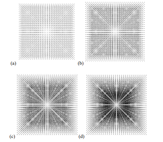
Figure 4: Face View with Different Numbers of Layers: 5, 10, 20, 50 in (a)–(d), Resp
Figure 5 shows voxels in the widest radial corridors and illustrates how the corridors penetrate the cube volume. The planes of the corridors are (011), (001), (01¯1), and (010).
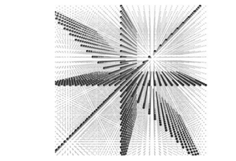
Figure 5: Voxels in Radial Corridors -45°, 0, +45°, and +90° Penetrate the Volume of the Cube (Slightly Deviated Face View)
Camera Displacement
The structure of the view image does not depend on parallel camera displacement (when the camera axis remains parallel to itself). Compare the overall corridor structure in Figures 6 and 7 with that in Figure 2(a).
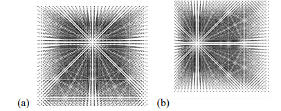
Figure 6: Face View with Camera Moved Horizontally (a) Along y’ Vertically Up, (b) Along x’ to the Right
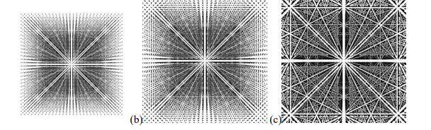
Figure 7: Different Distances (Camera Moved Along z’ to the Center of the Cube)
Some details may appear/disappear in each particular position, but the overall structure, including the relative locations of corridors and their intersections, remains unchanged. So, the parallel camera displacement is not essential.
Calibration
The angles of the widest corridors in the face view can be found by exploring the top facet of the cube or a layer parallel to the horizontal plane (001) viewed from a direction slightly deviated from [100]. This is called calibration. Particularly, the voxels in the top layer are arranged in a regular square grid. The camera looks slightly above the plane, almost along the grid axis. The picture resembles Euclid’s orchard [33]. Three corridors are clearly visible: one radial corridor in the middle and two symmetric lateral corridors, parallel to the radial one; see Figure 8.

Figure 8: Three Corridors in Plane (001)
Figure 9 shows how the nearest voxels are “connected” along the lateral corridor.
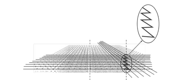
Figure 9: Two Corridors in the Top Layer with the Horizontal Angles 0 and 27° (= arctan (1/2)) From the Camera Axis
In the view perpendicular to the (001) plane (along [001]), Figure 10 shows the voxel grid.

Figure 10: Zigzag Line in the (001) Plane and Lengths of Legs
Figure 10 shows the number of voxels in each leg on the right side. Counting the grid voxels along the legs of the zigzag line in Figure 10 indicates that the arctangent of this angle equals 1/2. Based on that, we found that the angle of each side corridor is arctan (1/2) from the camera axis [17]. So, in angular units, the distance between the corridors is 1/2.
Symmetry implies that lines also run at the angle of -arctan (1/2). Therefore, it is reasonable to measure the view images in angular units, the arctangent units (ATU); see Figure 11.

Figure 11: Face View Calibrated in Arctangent Units (ATU)
There are several "focus" points on the axes — locations where non-radial corridors intersect the axes. Calibration makes it possible to obtain numerical values for these points.
Although we obtained only two points during calibration, we can apply the calibration results to any values, including intermediate ones, as well as to any view and any direction, including the polar radius.
Coordinate System
After calibration, we can use the orthogonal Cartesian system (x, y) based on the arctangent of the angle in the horizontal and vertical directions or the equivalent polar system (r, φ) with the angle φ measured from the abscissa; see Figure 12. The origin of the view image is on the camera axis.

Figure 12: Coordinate Systems
Mostly we use Cartesian coordinates between -1/2 and +1/2 ATU. The corresponding angular range of θ is (-27°, 27°), which means a “normal” camera lens (neither telephoto nor fisheye).
The Cartesian coordinates x and y correspond to the Euler angles α and β; the angle φ corresponds to the Euler angle γ [21,22].
We also use the angle θ from the camera axis, as in the spherical system. Note that the ray at θ is the diagonal of the rectangle built on the camera axis and the polar radius. Note also that the local x’-axis is horizontal.
Result
Structure of Corridors
Figure 13 shows the face view with axes calibrated in ATU units.

Figure 13: Face View of the Voxel Cube with Calibrated Axes
In the face view image, the most noticeable features are the radial rays (corridors). Due to symmetry, all 4 quadrants are identical.
Figure 14 shows the widest radial corridors in the first quadrant.

Figure 14: Radial Corridors (First Quadrant)
Radial Corridors
The angles of corridors can be identified in several ways: using the Radon and Hough transforms, as well as visually (based on the calibrated focus points) [17,34-36].
The dots in the sinogram (the result of the Radon transform) show the corridor locations; cross-sections of the sinogram show details, as shown in Figure 15.
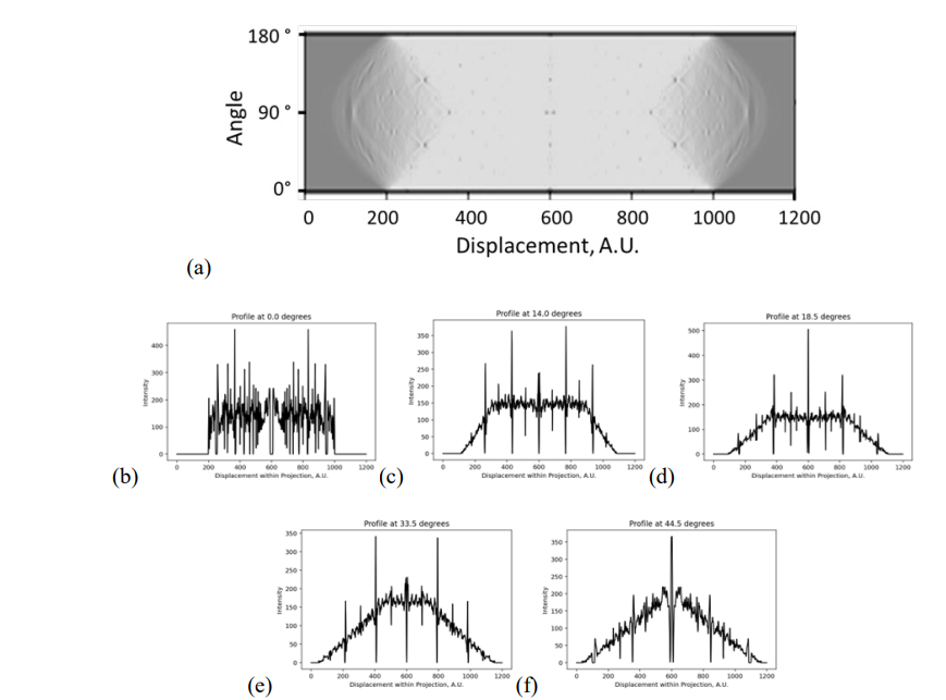
Figure 15: (a) Radon Sinogram and (b)-(f) its “Horizontal” Cross-Sections at Particular Angles 0°, 14°, 18.5°, 33.5°, 44.5°
The following Table 1 lists the corridor angles identified using the Radon transform.
|
0 |
206 |
251 |
303 |
321 |
372 |
400 |
426 |
463 |
484 |
502 |
512 |
595 |
|
|
|
|
|
-50.81 |
-45.00 |
-38.29 |
-35.96 |
-29.38 |
-25.76 |
-22.40 |
-17.63 |
-14.91 |
-12.59 |
-11.30 |
-0.58 |
radon |
|
|
|
|
|
-45.00 |
|
-33.69 |
|
-26.57 |
-21.80 |
|
|
|
|
0.00 |
expect |
|
|
|
|
|
0.0% |
|
6.3% |
|
3.1% |
2.7% |
|
|
|
|
|
|
|
|
|
|
|
|
|
|
|
|
|
|
|
|
|
|
|
|
|
|
14.04 |
181 |
186 |
262 |
434 |
599 |
|
|
|
|
|
|
|
|
|
|
|
|
-54.04 |
-53.39 |
-43.58 |
-21.37 |
-0.06 |
|
|
|
|
|
|
|
|
|
|
|
|
|
|
-44.13 |
-25.88 |
0 |
|
|
|
|
|
|
|
|
|
|
|
|
|
|
1.3% |
21.1% |
|
|
|
|
|
|
|
|
|
|
|
|
|
|
|
|
|
|
|
|
|
|
|
|
|
|
|
|
|
18.43 |
163 |
173 |
181 |
184 |
380 |
490 |
596 |
|
|
|
|
|
|
|
|
|
|
-56.36 |
-55.07 |
-54.04 |
-53.65 |
-28.34 |
-14.14 |
-0.45 |
|
|
|
|
|
|
|
|
|
|
|
|
|
-51.67 |
-32.31 |
|
0 |
|
|
|
|
|
|
|
|
|
|
|
|
|
3.7% |
14.0% |
|
|
|
|
|
|
|
|
|
|
|
|
|
|
|
|
|
|
|
|
|
|
|
|
|
|
|
|
33.69 |
159 |
167 |
172 |
192 |
213 |
222 |
411 |
503 |
599 |
|
|
|
|
|
|
|
|
-56.88 |
-55.85 |
-55.20 |
-52.62 |
-49.91 |
-48.74 |
-24.34 |
-12.46 |
-0.06 |
|
|
|
|
|
|
|
|
|
|
|
|
|
-47.9689 |
-29.0171 |
0 |
|
|
|
|
|
|
|
|
|
|
|
|
|
|
1.6% |
19.2% |
|
|
|
|
|
|
|
|
|
|
|
|
|
|
|
|
|
|
|
|
|
|
|
|
|
|
45 |
140 |
156 |
162 |
178 |
192 |
208 |
230 |
236 |
275 |
355 |
405 |
436 |
477 |
501 |
593 |
|
|
-59.33 |
-57.27 |
-56.49 |
-54.43 |
-52.62 |
-50.55 |
-47.71 |
-46.94 |
-41.90 |
-31.57 |
-25.11 |
-21.11 |
-15.82 |
-12.72 |
-0.84 |
|
|
|
|
|
-54.74 |
|
|
|
|
|
-35.26 |
|
|
|
|
0 |
|
|
|
|
|
0.6% |
|
|
|
|
|
11.7% |
|
|
|
|
|
Table 1: Angles from the Radon Transform
The Hough transform shows the corridors in a different form. Figure 16 shows the Hough angles.
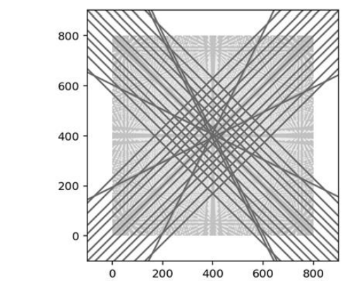
Figure 16: Hough Transform (One Option)
Table 2 shows the recognized angles.
|
Hough 1 |
0 |
1/4 |
1/3 |
1/2 |
|
2/3 |
3/4 |
|
|
1 |
|
Hough 2 |
|
|
|
|
3/5 |
|
|
4/5 |
5/6 |
|
Table 2: Angles from Hough transform
Thus, the radial corridors begin at the origin and extend along polar angles that have rational tangents,

where p, q are integers 0, 1, 2, 3, …
Table 3 lists the polar angles φ of the visually observed radial corridors.
|
p |
0 |
1 |
1 |
1 |
1 |
2 |
1 |
3 |
2 |
3 |
4 |
5 |
|
|
q |
|
5 |
4 |
3 |
2 |
3 |
1 |
2 |
1 |
1 |
1 |
1 |
0 |
|
tan φ |
|
1/5 |
1/4 |
1/3 |
1/2 |
2/3 |
1 |
1 1/2 |
2 |
3 |
4 |
5 |
|
|
|
0 |
0.20 |
0.25 |
0.33 |
0.50 |
0.67 |
1.00 |
1.50 |
2.00 |
3.00 |
4.00 |
5.00 |
∞ |
|
φ |
0 |
11.31 |
14.04 |
18.43 |
26.57 |
33.69 |
45.00 |
56.31 |
63.43 |
71.57 |
75.96 |
78.69 |
90 |
|
negative Inverse |
-∞ |
-5.00 |
-4.00 |
-3.00 |
-2.00 |
-1.50 |
-1.00 |
-0.67 |
-0.50 |
-0.33 |
-0.25 |
-0.20 |
0 |
|
|
|
-5 |
-4 |
-3 |
-2 |
-1 1/2 |
-1 |
-2/3 |
-1/2 |
-1/3 |
-1/4 |
-1/5 |
|
Table 3: Visually Observed Radial Corridors
Note the values 0.67 and 1.50 (which have the same absolute value but opposite signs), located at the corners of the square surrounding the 45° angle.
Parallel and Perpendicular Corridors
Other corridors are parallel to the radial rays; some are
perpendicular. Each radial corridor has at least one parallel and one perpendicular neighbor displaced from the origin. Some perpendiculars are indicated in Table 3 in bold font.
Figure 17 illustrates the parallel and perpendicular corridors.
(a) (b)

Figure 17: Corridors of the Face View: (a) Parallel and (b) Perpendicular to the Radial Corridors
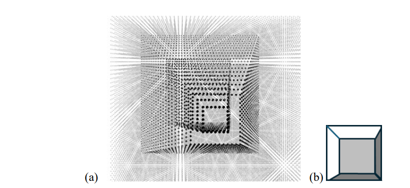
Figure 18 shows how perpendicular corridors penetrate the volume along the facets of pyramids.
The perpendiculars cross the radial rays at certain distances from the origin (along the polar radius, that is, at a certain angle θ from the camera axis). This is visible in cross-sections of the Radon sinogram. The following formula describes θ as the product of a constant 1/√s and a rational number K, which depends on the polar angle (or, equivalently, on integers p and q),

where
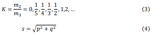
and p, q are from the definition of the angle φ.
The Appendix A provides examples of angles φ. Note that K is such that angle θ remains within the range of approx. 13° – 27°. (Recall the “normal” camera lens.)
Focus Points
The corridors connect the “focus” points on the axes. The calibration shows these focus points. The coordinates of the focus points can be described in rational numbers,
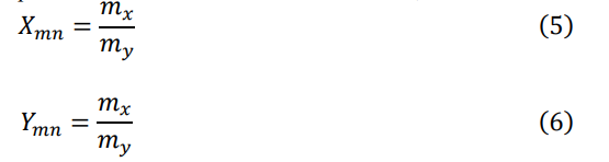
Tables 4 and 5 list the observed focus points on the x- and y-axes.
|
mx |
0 |
1 |
1 |
1 |
1 |
2 |
1 |
3 |
2 |
3 |
4 |
5 |
|
nx |
1 |
5 |
4 |
3 |
2 |
3 |
1 |
2 |
1 |
1 |
1 |
1 |
|
X (±) |
0 |
1/5 |
1/4 |
1/3 |
1/2 |
2/3 |
1 |
1 1/2 |
2 |
3 |
4 |
5 |
|
|
|
0.20 |
0.25 |
0.33 |
0.50 |
0.67 |
1.00 |
1.50 |
2.00 |
3.00 |
4.00 |
5.00 |
Table 4: Focus Points on the Abscissa
|
my |
0 |
1 |
1 |
1 |
1 |
2 |
1 |
2 |
|
ny |
|
5 |
4 |
3 |
2 |
3 |
1 |
1 |
|
Y (±) |
0 |
1/5 |
1/4 |
1/3 |
1/2 |
2/3 |
1 |
2 |
|
|
|
0.20 |
0.25 |
0.33 |
0.50 |
0.67 |
1.00 |
2.00 |
Table 5: Focus Points on the Ordinate
Note that most integer values in Tables 4 and 5 are ≤ 5, and rational numbers p/q and m/n in neighboring cells of the three Tables differ by less than a factor of two.
In principle, there are many combinations of rational angles for all possible corridors connecting all focus points on the two axes, from 1/5 to 2. However, in practice, we observed very few angles, and these had m = 1 or n = 1 with a couple of exceptions. Actually, they are listed in Table 3.
Discussion
The conditions for moiré fringes to appear in a cubic lattice are identical layers with identical spatial orientation (non-twist), a voxel size √2 times smaller than the period, and over four layers [17]. Thus, to reduce moiré patterns in a volumetric 3D cube, one could increase the voxel diameter. However, to observe larger-diameter voxels, the observation distance should increase [37].
So-called "anchor points" are not located at the vertices of a cube, as suggested in [17], but rather at the intersections of corridors—positioned at specific horizontal and vertical angles relative to the camera axis. For this reason, we performed a rigorous calibration in the current paper and do not use the term "anchor point.", although its definition could be refined.
If an observer has a preferred hemisphere, e.g., the wall behind blocks a full 360° view, the voxel size can vary along the z-axis [38,39]. Figure 19 shows the face view with different voxel diameters.
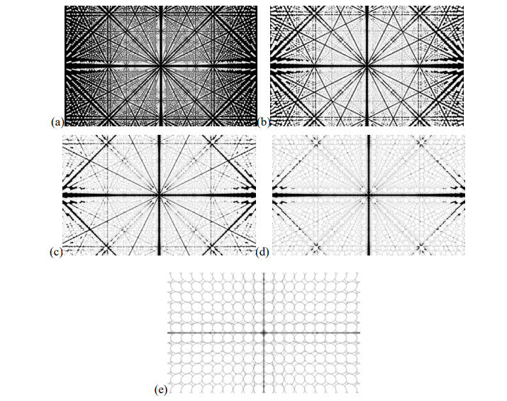
Figure 19: Image of the Face View with Different Voxel Sizes in (a)-(e): 0.2, 0.3, 0.4, 0.5, 1
No corridors remain at d = 1, but no image is possible, except for a planar 2D image in the nearest plane! Figure 20 shows another example with the voxel size increased by 0.1% at each step along z. The corridors in the central part of the view almost disappear, except for the widest ones at 0 and 45°.
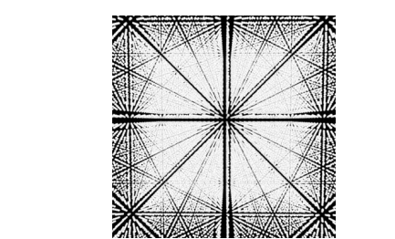
Figure 20: Non-Identical (increased) Size of Voxels Along the z-Axis
In the next visual experiment (see Figure 21), we randomized the locations of voxels to minimize the moiré effect as in [40].
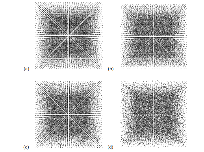
Figure 21: (a), (b) Random x -Locations (Randomization 0.5 and 1.0 of Cell Size). (c), (d) Random xy -Locations (0.5, 1.0 Size)
Conclusion
We investigated the visual moiré effect in a simple cubic lattice when viewed from a finite distance. This is the first part of the study, where we examined the face view (along the [100] axis) in detail. We showed that parallel camera displacement has no significant effect on the visual image (except for minor details). The characteristic angles of the "corridors" are independent of the lattice constant and the distance to the camera; consequently, these corridors permeate the entire volume of the cube regardless of the number of layers (we provided a graphical illustration of radial and perpendicular corridors). This moiré effect is inherently multilayered: observing these patterns requires at least four or five layers. Detailed computer simulation based on Radon and Hough transforms confirms the moiré angles in the face view. The tangents of the radial corridors' inclination angles are rational numbers. Other corridors connect focus points (with rational coordinates) on the axes and run parallel and perpendicular to radial corridors. We derived equations for the focus points and perpendicular corridors and formulated the conditions for the emergence of moiré patterns in a multilayered 3D object. The results may apply to crystallography and to volumetric displays with static LEDs (with a mechanically fixed arrangement of voxels), where varying voxel size or using random voxel placement can minimize the moiré effect.References
- Amidror, I. (2009). The Theory of the Moiré Phenomenon: Volume I: Periodic Layers. Springer London.
- Bryngdahl, O. (1974). Moiré: formation and interpretation.Journal of the Optical Society of America, 64(10), 1287-1294.
- Creath, K., & Wyant, J. C. (1992). Moiré and fringe projection techniques. Optical shop testing, 2, 653-685.
- Saveljev, V. (2022). The Geometry of the Moiré Effect in One, Two, and Three Dimensions. Cambridge Scholars Publishing.
- Theocaris, P. S. (1967). Moiré topography of curved surfaces: the moiré method is extended to measure deflections and slopes in cylindrical and conical shells. Experimental Mechanics, 7(7), 289-296.
- Sciammarella, C. A., & Chiang, F. P. (1968). Gap effect on moiré patterns. Zeitschrift für angewandte Mathematik und Physik ZAMP, 19(2), 326-333.
- Saveljev, V., & Kim, S. K. (2010). Simulation of moiré effect in 3D displays. Journal of the Optical Society of Korea, 14(4), 310-315.
- Saveljev, V., Kim, S. K., & Kim, J. (2018). Moiré effect in displays: a tutorial. Optical Engineering, 57(3), 030803-030803.
- Saveljev, V., Son, J. Y., Kim, Y., Park, J. G., & Heo, G. (2020). Moiré patterns in non-parallel surfaces such as wedge. Journal of the Optical Society of America A, 37(2), 336-345.
- Saveljev, V. (2016). Moiré effect in cylindrical objects.Journal of the Korean Physical Society, 68(9), 1075-1082.
- Post, D., Han, B., & Ifju, P. (1997). High sensitivity moiré: experimental analysis for mechanics and materials. Springer .
- Chiang, F. P. (1979). Moiré methods of strain analysis.Experimental mechanics, 19(8), 290-308.
- Sciammarella, C. A. (1982). The moiré method—a review: The main developments in the area of moiré as a tool to measure displacements, contours, slopes and strains are reviewed and some typical applications are shown. Experimental mechanics, 22(11), 418-433.
- Patorski, K., KujawiÅ?ska, M. (1993). Handbook of the moiré fringe technique. Elsevier.
- Gao, Z., Konotop, V. V., Peng, R., Xu, Z., Yang, Z., & Ye, F. (2025). Low-dimensional compact states in 3D moiré lattices. Nature Communications, 16(1), 6306.
- Hurley, N., Kamau, S., Cui, J., & Lin, Y. (2023). Holographic fabrication of 3D moiré photonic crystals using circularly polarized laser beams and a spatial light modulator. Micromachines, 14(6), 1217.
- Saveljev, V. (2023). Moiré effect in multilayered 3D lattice.Applied Optics, 62(11), 2792-2799.
- Monaco, H. L., Viterbo, D., Scordari, F., Gilli, G., Zanotti, G., & Catti, M. (2002). Fundamentals of crystallography (Vol. 7).C. Giacovazzo (Ed.). Oxford: Oxford university press.
- Ashcroft, N. W., & Mermin, N. D. (1976). Solid state physics. Holt, Rinehart and Winston.
- Popov, I., & Besley, E. (2026). Three-dimensional moiré crystallography. arXiv preprint arXiv:2601.04971.
- Nolze, G. (2015). Euler angles and crystal symmetry. Crystal research and technology, 50(2), 188-201.
- Feuerbacher, M. (2021). Moiré, Euler and self-similarity–the lattice parameters of twisted hexagonal crystals. Acta Crystallographica Section A Foundations and Advances, A77(5), 460-471..
- Weisstein, E. W. (2025). Cubic lattice. MathWorld—A Wolfram Resource.
- Visual physics and mathematics/Crystal structures. (2024, February 1). Wikibooks. Retrieved October 2.
- Blundell, G., Schwarz, A. J. (2000). Volumetric Three-Dimensional Display Systems. Chap. 6. Wiley.
- Wyatt, D., & Wujanto, L. (2005). A volumetric 3D LED display. MIT, 6, 1-48.
- Rowe, A. (2012). Within an ocean of light: creating volumetric lightscapes. In ACM SIGGRAPH 2012 Art Gallery (pp. 358 365).
- iCubeSmart 8x8x32RGB. (2026).
- LED cube. (2026).
- Pimenta, W., & Santos, L. P. (2012). A comprehensive taxonomy for three-dimensional displays. WSCG'2012. (pp. 139-146).
- Blundell, B. G., & Schwarz, A. J. (2002). The classification of volumetric display systems: characteristics and predictability of the image space. IEEE Transactions on Visualization and Computer Graphics, 8(1), 66-75.
- Web VPython (glowsctipt). (2026).
- Weisstein, E.W. (2025). Euclid's orchard. MathWorld--A Wolfram Resource.
- Duda, R. O., & Hart, P. E. (1972). Use of the Hough transformation to detect lines and curves in pictures. Communications of the ACM, 15(1), 11-15.
- van Ginkel, M., Kraaijveld, M. A., van Vliet, L. J., Reding,E. P., Verbeek, P. W., & Lammers, H. J. (2003, June). Robust curve detection using a Radon transform in orientation space. In Scandinavian Conference on Image Analysis (pp. 125-132). Berlin, Heidelberg: Springer Berlin Heidelberg.
- Brandt, D., Nikishina, A. A., Bias, A., Günther, R., Hauser, A. E., Duda, G. N., ... & Niesner, R. A. (2025). Segmentation-free Radon transform algorithm to detect orientation and size of tissue structures in multiphoton microscopy images. Journal of Biomedical Optics, 30(8), 086001-086001.
- Saveljev, V. (2026). Combined Physical and Computational Simulation of the Moiré Effect in 3D Objects and Displays. In Intelligent Systems: From Data to Decisions (Ch. 5, pp. 93-122). Haliç Publishing House, Ä°stanbul, Türkiye.
- Bougdid, Y., & Sekkat, Z. (2020). Voxels optimization in 3D laser nanoprinting. Scientific Reports, 10(1), 10409.
- Ghankot, R. S., Singh, M., Desroches, S. T., Jester, N., Mahajan, A., Lorr, S., ... & Tommasini, S. M. (2025). Evaluating the effect of voxel size on the accuracy of 3D volumetric analysis measurements of brain tumors. Frontiers in Radiology, 5, 1618261.
- Xia, X., Zhuang, X., He, H., Wu, X., Zheng, H., & Yu, Y. (2025). Moiré-free and high-resolution light field 3D display based on random parallax barrier. Journal of Physics: Photonics, 7(3), 035009.
Appendix A: Parameters of Perpendicular Corridors
A1.Crystallographic Plane (001)
The plane's numerical parameters: p = 0, φ = 0; s = 1, √s = 1. This is the case of perpendiculars to the abscissa (ray φ = 0). So, their distances from the origin θ are actually the abscissas of the focus points with K = mx/nx; see Table A1. The cross-section of the cube along φ = 0 and perpendiculars in this cross-section are shown on the right side of Figure A1.
|
Coefficient K |
1/5 |
1/4 |
1/3 |
1/2 |
|
tan θ |
0.20 |
0.25 |
0.33 |
0.50 |
|
angle θ, deg |
11.31 |
14.04 |
18.43 |
26.57 |
Table A1: Perpendiculars in Plane (001)
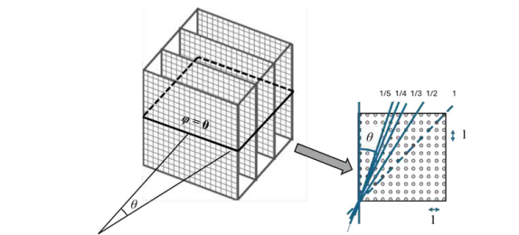
Figure A1: Corridors Perpendicular to the Abscissa and the Cross-Section φ = 0
A2. Crystallographic Plane (011)
The numerical parameters of the plane: p/q = 1/1, φ = 45°; s = 2, √s = 1.41. The angles of the perpendiculars are listed in Table A2. Figure A2 shows a graphical illustration.
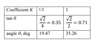
Table A2: Perpendiculars in Plane (011)

Figure A2: Perpendiculars to the Ray φ = 45° and the Cube Cross-Section
Crystallographic Plane (012)
The numerical parameters of the plane: p/q = 1/2, φ = 26.6°; s = 5, √s = 2.24. The angles of perpendiculars are listed in Table A3. Figure A3 is a graphical illustration.
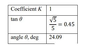

Table A3: Perpendiculars in Plane (012)
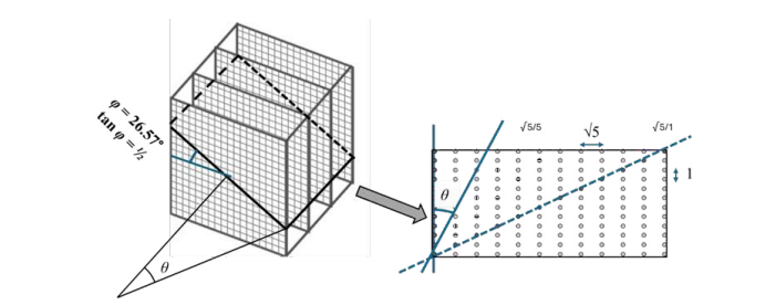
Figure A3: Perpendiculars and Cross-Section for φ = Arctan (1/2)
A4. Crystallographic Plane (013)
The numerical parameters of the plane: p/q = 1/3, φ = 18.4°; s = 10,
√s = 3.16. The angles of the perpendiculars are listed in Table A4. Figure A4 shows a graphical illustration.
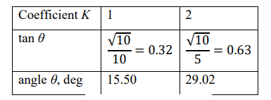
Table A4: Perpendiculars in Plane (013)
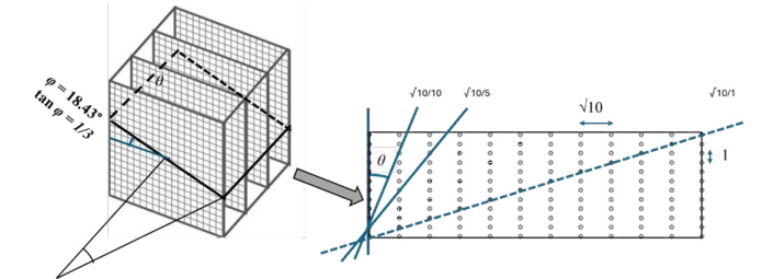
Figure A4: Perpendiculars and Cross-Section for φ = arctan (1/3)
A5. Crystallographic Planes (023) and (014)
The numerical parameters of plane (023) are: p/q = 2/3, φ = 33.7°; s = 13, √s = 3.61. The numerical parameters of plane (014) are: p/q = 1/4, φ = 14.0°; s = 17, √s = 4.12. The angles of perpendiculars are listed in Tables A5 and A6.
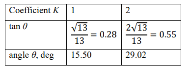
Table A5: Perpendiculars in Plane (023)
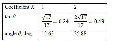
Table A6: Perpendiculars in Plane (014)