Reduction of GHG Emissions: Air Quality Improvement in Urban Areas

Introduction

Urban zones are the most sensitive to pollutant emissions because of the surface restriction and the concentrated population. Among the many factors that contribute to impoverish the air quality is the road traffic [1,2]. Public and private transportation use combustion engines to propel the vehicles with the only exception of pure electric vehicles (EVs) nevertheless, this last category represents a minimum percentage of the vehicle fleet [3,4]. The continuous increase of pollution level in populated cities leads the politicians to adopt regulations to reduce GHG emissions and improve the air quality; traffic restrictions and coercive measures are, among others, the most frequent decisions [5,6]. The elimination of combustion engines represents the definitive solution for the pollution problem; however, the economic impact of this decision slows down the implementation of this measure [7-9].

A less restrictive policy is the synthetic fuels use for combustion engines like the biodiesel; however, the use of biodiesel shows collateral damages or unexpected consequences, which may result in drawback effects on the environment [10-15]. Bio-gasoline is an alternative for GHG emissions reduction for vehicles equipped with gasoline combustion engines because of higher engine performance [16,17]. Bio-oil is a promising option to replace conventional fossil fuels to reduce gasses emissions [18,19]. Nevertheless, all the mentioned fuels suffer from gasses emissions to a greater or lesser extent, which, despite contributing to reducing greenhouse gas emissions, does not solve the problem in the long term [20-24].

In past decades, automotive industry proposes the use of hydrogen combustion engines (HCE) [25-27]. to which many people devoted specific studies and research [28-34]. The advantage of using hydrogen as fuel in combustion engines is the absence of GHG emissions, since the hydrogen combustion only produces water; however, the hydrogen suffers from a low energy density in gaseous form, what forces to liquefying it to increase the mass density, thus, the specific power this process, however, requires a low temperature to maintain hydrogen in liquid state, around -253º C, which represents a technological challenge, especially in mobile storage tanks [35-37].

We solve the technological problems derived from the liquid hydrogen use operating with its gaseous form; this solution, although technically more feasible, requires compressing the hydrogen at high pressure, up to 700 bar, to get the appropriate mass density [38-40]. Compressed hydrogen tanks do not represent a technical problem but for security since hydrogen at high pressure may ignite or explode easier than at ambient pressure [41,42]. On the other hand, hydrogen tend to self-ignite or explode during discharge what makes its use hazardous and technically complicated [43,44].

Avoiding the use of hydrogen and considering that full electric vehicles still require some time for a complete implementation, we return to the question on reducing the GHG emissions in combustion engines. In this work we propose a novel solution, which is to limit the fuel consumption by adapting the driving mode to a more conservative way. The limitation of fuel consumption means a lower gasses emission level, contributing to maintaining or improving air quality, especially in contaminated urban zones.

Fuel Consumption Reduction

The most effective way to reduce fuel consumption is double, limiting the vehicle speed and reduce acceleration when necessary. Indeed, since fuel consumption depends on the required energy to propel the vehicle, and the power depends on the propelling force and average speed, we lower the energy demand by reducing both. On the other hand, propelling force depends, among other factors, on vehicle acceleration and speed; therefore, a limitation in both dynamic parameters, speed and acceleration, reduces the required force, thus the power and energy consumption. Because carbon emissions directly relate to fuel consumption, we reduce CO2 emissions by lowering fuel consumption.

Considering the many vehicles operating daily in urban areas, the carbon emissions due to road traffic represent a high environmental impact, especially in city downtown where traffic is more concentrated and air venting is more complicated. Since the urban route distances are currently short, a limitation in the average vehicle speed does not represent high impact on the route time. We use daily urban routes distance according to a reference statistical analysis (Figure 1) nevertheless, we expand the urban route distance to a maximum of 25 km to cover all the vehicle fleet running in daily urban routes [45].

Figure 1: Distribution of Urban Trip Distances in the Eu Based on Miscellaneous Data Sources [45]

To extend the statistical analysis shown in figure 1 to the maximum percentage of 100%, we correlate the values to a third-degree poly- nomial function, obtaining the following expressions:

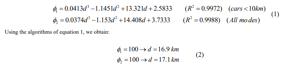
Therefore, we extend the daily route distance to 17 km. We use a distance interval of 2.5 km to avoid excessive data number. Figure 2 shows the time increase as a function of the daily route distance and vehicle speed reduction for the various average vehicle speed. We notice that the time reduction represents, in some cases, a sig- nificant delay in the daily route duration, which may incline the driver not to reduce the average speed; therefore, we must select the vehicle speed reduction according to an acceptable percentage of time increase regarding the daily urban route duration. Setting up a maximum increase of 25% in the daily route duration, suitable for many drivers [46-48]. we can determine the maximum vehicle speed reduction for every average vehicle speed (Figure 3).

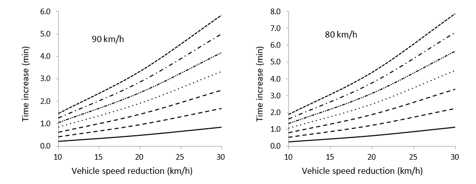
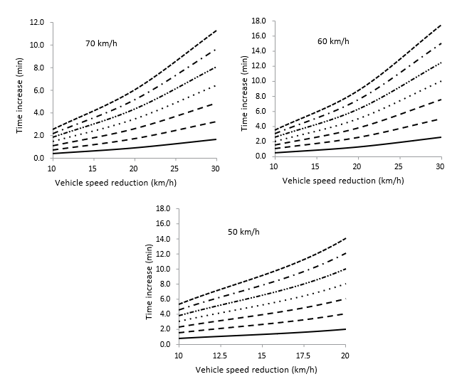
Figure 2: Time Increase as a Function of the Vehicle Speed Reduction and Daily Urban Route Distance

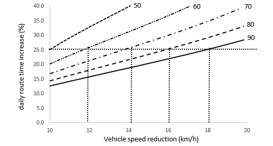
Figure 3: Maximum Vehicle Speed Reduction for a Maximum Set Up Time Enlargement

We notice that the maximum speed reduction represents a 20% of the vehicle speed average value when considering a time enlarge- ment of 25%. We also realize that no speed reduction is applicable for vehicle speed 50 km/h and slower. The analysis of the simu- lated study for time enlargement due to vehicle speed reduction shows that we can reduce car velocity by a 20% without signifi- cant delay in the daily route duration, which implies reducing the carbon emissions and improving air quality in urban areas. For practical reasons we operate the average vehicle speed within a range of around 20% to classify the driving mode in three groups, sport, normal and eco mode, for high, medium and low car veloc- ity between 70 and 90 km/h, 50 to 70 km/h and below 50 km/h, respectively.

On the other hand, the comparative analysis applies to three driving patterns: sport or aggressive, normal or moderate, and eco or conservative; the acceleration values corresponding to the three driving modes are set up at 3.5 m/s2, 2.5 m/s2 and 1.5 m/s2, re- spectively.

Fundamentals

Driving consists of three dynamic processes, acceleration, con- stant speed and deceleration, which may happen in flat, ramped or sloping terrain. Combining the three driving modes with the oro- graphic configuration of the terrain produces nine different cases, with specific dynamic properties for each one.

Required energy to propel a vehicle derives from the classical equation of the Dynamics:

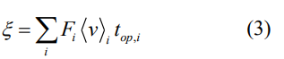
Where F is the dynamic force, the average vehicle speed, and top the event duration. The sub-index i accounts for the i-segment of the route.

In conventional vehicles equipped with Internal Combustion En- gine, all the segments of the route use fossil fuel to propel the car; however, in hybrid (HEV) and plug-in hybrid electric vehicles (PHEV), only a fraction of the time the combustion engine oper- ates while for the rest of the time the car runs on electric energy, which does not emit greenhouse gasses. On the other hand, electric vehicles equip an Energy Recovery System (ERS), which uses the loss of kinetic energy to generate electricity, reversing the electric engine and making it playing as electric generator. In case of full electric vehicles (EV), since they do not use a combustion engine at any time, all GHG emissions by ICE cars are avoided.

The electric engine time use in HEV and PHEV depends on the driving pattern, average vehicle speed and battery management system (BMS). BMS currently applies to charge process, but its application to battery discharge is critical for battery performance optimization. Indeed, the battery suffers from quick discharge if battery powers the vehicle during the acceleration process when the power demand increases, and its capacity lowers, thus reduc- ing the discharge time and the battery autonomy [49].

Electric vehicles operate under different protocols depending on the configuration: mild hybrid (MHEV), hybrid (HEV) or plug-in hybrid (PHEV). In mild hybrid electric vehicles, the engine always powers the car, assisted by a powerful battery when accelerating; this operational mode limits the power demand and reduces the engine workload. In full hybrid electric vehicles (HEV), the car runs on electric power over a short distance, with the battery taking over the ICE. Plug-in hybrid electric vehicles (PHEV) operate in a similar way to HEV [50].

An alternative protocol uses the battery to power the electric vehi- cle at starting or low speed to accelerate the car; in acceleration or uphill road the electric and combustion engine operates in parallel to maximize power supply and minimize fossil fuel consumption. In constant speed mode the electric and combustion engine alter- nates powering the vehicle, whichever is the most efficient. Final- ly, in deceleration or road downhill, neither the combustion nor electric engine works since the regenerative braking activates and the electric engines reverses to generate electricity to charge the battery [51].

Electric vehicles recover energy during deceleration or braking; therefore, the net energy balance for electric cars is:

F represents the global dynamic force exerted on the vehicle, where sub-indexes j=1,2,3 account for uphill, horizontal and downhill road, and k=a,b,c for acceleration, constant speed and deceleration, respectively; v is the average vehicle speed, with sub-indexes o and f accounting for initial and final state of a route segment, d is the segment travelled distance and τ the correspond- ing time. Cr and ηr are the recovery energy coefficient and battery charge efficiency.

It is necessary to compute the operating time in electric mode if we deal with hybrid and plug-in hybrid electric vehicles, which is difficult to determine since it depends on driving pattern and on electric vehicle configuration. Because there are too many configu- rations, we standardize the electric operating mode through a time factor, representing the fraction of the global time where vehicle runs in electric mode. In such a case, equation 4 converts into:

F_e is the time factor, which depends on the driving pattern and on the vehicle speed.

Time Factor

To determine the time factor, we use the database from previous developed experimental studies on different commercial hybrid and plug-in hybrid electric vehicles [52-55]. The studies analyze the electric mode operational time in hybrid and plug-in hybrid electric vehicles for different route types, urban, peripheral and intercity, and for variable driving conditions, vehicle speed and driving pattern.

The minimum covered distance for every type of route is 6500 km, combining all driving conditions in the entire group of tests. Low speed is characteristic of urban routes; intermediate and high correspond to peripheral and intercity routes. Nevertheless, we de- velop short tests for medium and high speed in urban routes. We also test the different driving patterns, high, medium and low ac- celeration, corresponding to sport (aggressive), current (moderate) and eco (conservative) driving mode during each of the driving tests. To properly analyze the dependence of time factor on vehicle speed and acceleration, we devote different tests for every specific driving condition. Table 1 shows the results of the various studies.

Table 1: Time Factor for HEV and PHEV in Urban Route [52-55].

We take the average vehicle speed for testing. The registered speed values are within a deviation range of 3-5 km/h due to the accuracy of the vehicle speedometer. We can apply individual time factor values in equation 5. The analysis of results from table 1 shows that, on average, plug-in hybrid vehicles use the electric mode 2.6 times longer than hybrid electric vehicles, considering all driving patterns and routes. Time factor ratio between PHEV and HEV varies from a minimum of 1.684 for low speed, eco mode in urban route, to a maximum of 8.75 for high speed, sport mode in urban route.

Simulation

To evaluate the influence of the driving conditions on the carbon emissions, we run a simulation for the different vehicle type run- ning in urban areas: combustion engine, diesel or gasoline, and electric cars, HEV, PHEV and EV. To avoid deviations due to the vehicle structure or road configuration, we consider a prototype with specific mass, aerodynamic coefficient, front area and tire contact zone so that we operate with common vehicle characteris- tics. Table 2 shows the vehicle prototype characteristics.

Table 2: Characteristics of the Vehicle Prototype

The simulation applies to a set up road configuration with uphill, horizontal and downhill segments with vehicle submitted to differ- ent driving conditions, acceleration, constant speed and decelera- tion. The unique difference in vehicle performance is the recovery energy in EVs.

We use a prototype road configuration defined in a previous work consisting in 13 segments distributed as follows: four horizontal, two uphill, two horizontals again, two downhill, and three hori- zontals anew [65]. (Figure 4). The number inside the circle corre- sponds to the vehicle speed in km/h.

                                               Figure 4: Layout of the Prototype Urban Route

Since we use the vehicle speed average value for calculating the required power and the energy consumption, we consider that the veloc- ity evolves linearly when the car accelerates or decelerates because the travelled distance for any segment is short. Applying Dynamic equations, we obtain (Table 3).

                                                                                                            segment

                                   1        2        3         4          5         6         7         8        9        10       11      12      13

Legend: <v>: average vehicle speed (m/s); a: Acceleration (m/s²); d: distance (m); t: time (min): θ: road tilt angle (º)

Table 3: Dynamic Parameters of the Prototype Daily Urban Route

To adapt vehicle speed to the classification of Table 1, we establish the following correspondence: slow from 0 to 50 km/h, medium from 50 to 70 km/h, and high from 70 to 90 km/h, according to the statement in the analysis of time enlargement for vehicle speed reduction.

CO₂ Emissions

Carbon emissions proceeds from the fossil fuel combustion; CO2 rate depends on the fuel type, according to data presented in Table 3. To calculate the global carbon emissions, we apply the follow- ing expression:

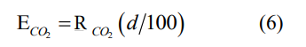
Where R CO2 is the carbon emissions rate shown in Table 4?

Table 4: Fuel Type GHG Emissions [66-70].

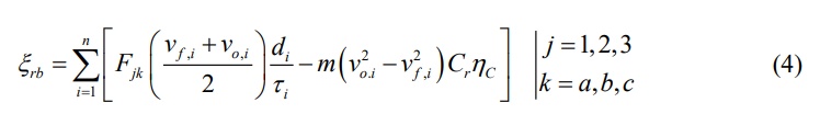
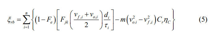
Using equations 4 and 5, and data from Table 2, we obtain the energy demand for ICE cars in standard units

Now, applying the time factor to energy consumption rate for EVs (Table 5):

Table 5: Energy Consumption and Energy Saving in Hev, Phev and Ev for the  Prototype Urban Route

We notice that using HEV reduces the energy by 15.4% on aver- age, while the reduction when using PHEV is 47%. Obviously, the reduction when using EV is 100%. If we analyze the driving pattern, the average reduction is 48.4%, 51.8% and 54.6% for the sport, normal and eco mode, respectively.

To convert energy in fuel consumption, we use the fuel combus- tion power and the engine and transmission efficiency according to the expression:

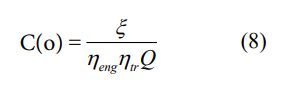
ξ is the energy demand, Q the fuel combustion power, and η the efficiency with sub-indexes end and tr for engine and transmission.

We show standard average values for engine and transmission efficiency and fuel combustion power for EV and ICE cars in Table 6.

Table 6: Engine and Transmission Efficiency and Fuel Combustion Power for Ice Cars and Electric Vehicles [71-73].

Transmission efficiency in electric vehicles corresponds to the me- chanical transmission when using ICE; therefore, it matches the value for ICE cars. It is not applicable to full electric vehicles be- cause they do not use conventional mechanical transmission.

We use the gasoline combustion power for HEV and PHEV since most hybrid and plug-hybrid electric vehicles use gasoline ICE. The same statement applies for the engine efficiency.

Using equation 6 and tables 5 and 6:

Table 7: Fuel Consumption for Ice Cars and Electric Vehicles

(1) Sport driving mode; (2) normal driving mode; (3) eco driving mode Now, converting the fuel consumption to GHG emissions, we have (Figures 5 to 7):

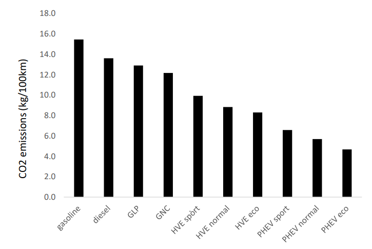
Figure 5: Co₂ Emissions by Type of Vehicle and Driving Mode

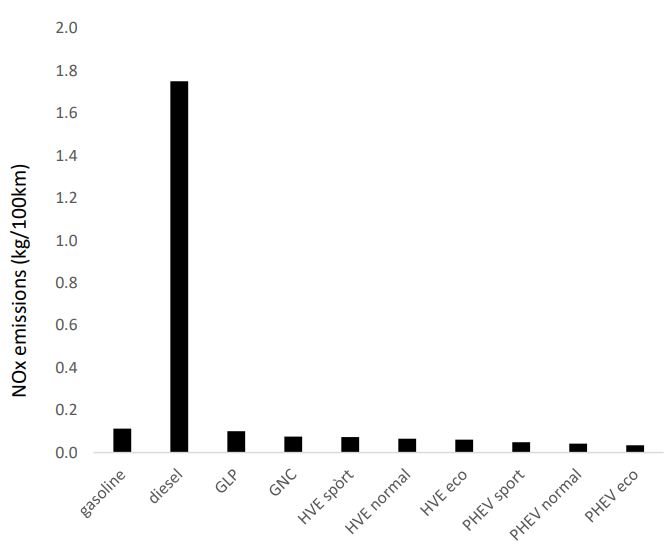
Figure 6: Nox Emissions by Type of Vehicle and Driving Mode

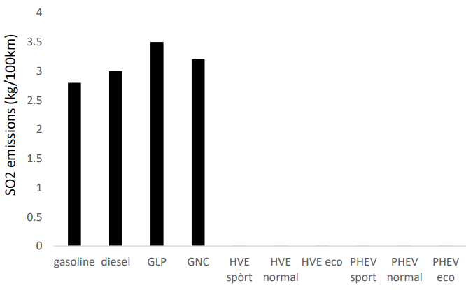
Figure 7: So₂ Emissions by Type of Vehicle and Driving Mode

The analysis of GHG emissions shows that electric vehicles drastically reduces the SO2 and NOx emissions and contribute to a reduction of more than 45% in CO2 emissions, on average, with a maximum of 53% for the eco driving mode and a minimum of 39% for the sport mode.

Environmental Evaluation

Greenhouse gasses analyzed in this study increase the pollution level and contribute to the climatic change the individual ef- fect, however, differs from one gas to another since the impact depends on several factors: global emissions, specific impact, and normalization and evaluation factor [74-76].

To harmonize the environmental impact of any specific green- house gas, we should define a reference parameter like the GHG assessment framework, which is a standardized method for assessing the environmental aspects and potential impacts associated with all the intervening factor in the global effect of a GHG [77,78].

Impact assessment consists of four steps [79,80].

• Selecting the impact category

• Classification and LCI results assignment to the impact category

• Characterization: calculation of the category indicators • Normalization: determination of the category indicator value regarding the reference information

• Grouping: sorting or ranking the indicators

• Weighing: assignment of the specific weigh or importance to the potential influence factors

• Global influence value

We can summarize all factors listed above in a simplified mathe- matical expression as [81].

E is the gas global emissions and fch. fN and fev are the characteriza- tion, normalization and evaluation factor, respectively.

Since we already know the global emissions previously calculated, we should pay attention to the other three factors, which depend on the pollutant agent, the affected population and the collateral effects like biodiversity losses, increasing population death rate and others [82-95].

We classify GHG according to which environmental aspect influ- ence global warming, eutrophication, acidification, ozone layer reduction, winter mist and smog creation, heavy metal deposition, damaging radiation, etc. In this sense, the GHG emissions studied in this paper mainly affects to the global warming (CO2 and NO2) and acidification (SO2) [96-102].

From the point of view of global warming, we characterize carbon dioxide with a factor 1 while the nitrox dioxide characterizes with index 270 [103]. The influence of Sulphur dioxide on the global warming is similar to the carbon dioxide, with a characterization factor of 2 [104].

The normalization factor depends on the equivalent amount per inhabitant, which expresses how much gas emissions correspond to a single person; mathematically

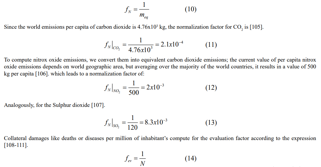
We realize that carbon dioxide represents the most dangerous agent to the environment, with an ecological evaluation factor more than two hundred times higher than the nitrox oxide and almost 3500 times higher than the Sulphur dioxide.

Combining these values with the simulation results in the present study, Figures 5, 6 and 7, we obtain the global impact of the three GHG studied in this paper (Table 8).

Table 8: Global Environmental Impact of Co₂, No₂ and So₂ for the Simulation Case

Comparing values from table 8, we notice ICE cars produce a 50% more environmental impact than HEV and 140% more than PHEV regarding carbon dioxide, with the gasoline as the most influencing factor. We also notice there is not a great deviation between the impact values from different ICE engines. If we average the impact generated by internal combustion engines, the resulting value is 25022, with a maximum deviation of 14%. On the other hand, HEVs have a 60% greater impact than PHEV.

If we deal with nitrox oxides, ICE cars produce 7.8 times more impact than HEVs and 12.4 times more than PHEVs. In this case, diesel engines are responsible of most of the environmental impact, with an impact ratio of 18.3 regarding the average value of the others ICE engines. As in the carbon dioxide case, HEV has 60% greater impact than PHEV.

The results from the analysis of the Sulphur dioxide impact has on the environment produce much higher differences between ICE cars and EVs; internal combustion engines generate almost 2000 times more impact than EVs, with similar values between the different engine types. The average impact value of ICE cars is 1.656, with a maximum deviation of 12%. The impact ratio of HEV to PHEV maintains in 60%.

Conclusions

We develop a study to determine the influence of electric vehicles on the environmental impact in urban areas compared to the internal combustion engine cars. The study analyzes the greenhouse gasses emissions of four type of conventional cars powered by gasoline, diesel, GLP and GNC, and three electric vehicle types: hybrid (HEV), plug-in hybrid (PHEV) and full EV. The analysis results show that using electric vehicles improve air quality in urban areas due to significant GHG emissions reduction.

We apply dynamic conditions to a standard urban route that includes uphill, horizontal and downhill road segments where every segment characterizes by a vehicle speed and acceleration and a road tilt. The application of dynamic conditions results in a lower fossil fuel consumption in electric vehicles despite the higher weight because of the powering battery. The fuel consumption reduction redounds in a lowering of fossil fuel energy use, which depends on the driving pattern and type of electric vehicle; the energy saving varies from a minimum of 6.8% for sport driving mode in HEVs to a maximum of 56.1% for eco mode in PHEVs. Full electric vehicles (EVs) contribute to save 100% fossil fuel energy.

The use of electric vehicles significantly lowers the greenhouse emissions, with an average reduction of more than 45% of carbon dioxide emissions and drastic reduction of NOx and SO2, with a lowering factor of 89.5% and 95.7%, on average, for these two gasses. GHG emissions lowering also depends on the electric vehicle type and driving pattern, with the EV as the environment friendliest car. HEV and PHEV are also more respectful with urban environment, with carbon dioxide reduction rate of 39% and 53%, and NOx and SO2 lowering rate of 88.2% and 95.2% for the HEV, and 90.7% and 96.2% for the PHEV.

Regarding the environmental impact, especially in urban areas, driving pattern is the most influencing factor; limiting vehicle speed and acceleration reduces GHG emissions significantly. Acceleration greatly influences the reduction of GHG emissions more than vehicle sped. Traffic regulations to this goal improve the air quality and reduce greenhouse emissions. A feasible solution to apply these measurements is the car control system implementation that regulates the vehicle acceleration and velocity in urban zones

An environmental impact analysis of the different type of internal combustion engines and electric vehicles results in a higher value for ICE cars regarding EVs. ICE cars are 50% more environmental impact than HEV and 140% more than PHEV regarding carbon dioxide, 7.8 times more impact than HEV and 12.4 times more than PHEV if we deal with nitrox oxides, and near 2000 times more for Sulphur dioxide.

Environmental impact of ICE cars is similar for CO2 and SO2; however, for nitrox oxides the diesel engines produces 18.3 times more impact than other ICE cars. Hybrid electric vehicles show a constant ratio of 60% higher impact than plug-in hybrid vehicles. Full electric vehicle does not produce environmental impact as far as its operational mode.

References

1. Briggs, D. (2003). Environmental pollution and the global burden of disease. British medical bulletin, 68(1), 1-24.
2. Laña, I., Del Ser, J., Padró, A., Vélez, M., & Casanova-Mateo,C. (2016). The role of local urban traffic and meteorological conditions in air pollution: A data-based case study in Madrid, Spain. Atmospheric Environment, 145, 424-438.
3. Pérez, J., de Andrés, J. M., Borge, R., de la Paz, D., Lumbreras, J., & Rodríguez, E. (2019). Vehicle fleet characterization study in the city of Madrid and its application as a support tool in urban transport and air quality policy development. Transport Policy, 74, 114-126.
4. What Percentage of Cars on the Road Are Electric in the Cities Worldwide. Energy5 your way. 9 November 2023. https://energy5.com/what-percentage-of-cars-on-the-road- are-electric-in-cities-worldwide.
5. Khreis, H., Sanchez, K. A., Foster, M., Burns, J., Nieuwenhuijsen, M. J., Jaikumar, R., ... & Zietsman, J. (2023). Urban policy interventions to reduce traffic-related emissions and air pollution: A systematic evidence map. Environment International, 172, 107805.
6. Gärling, T. (2007). Effectiveness, public acceptance, and political feasibility of coercive measures for reducing car traffic. In Threats from car traffic to the quality of urban life: Problems, causes and solutions (pp. 313-324). Emerald Group Publishing Limited.
7. Fageda, X., Flores-Fillol, R., & Theilen, B. (2022). Price versus quantity measures to deal with pollution and congestion in urban areas: A political economy approach. Journal of Environmental Economics and Management, 115, 102719.
8. Chiesa, M., Perrone, M. G., Cusumano, N., Ferrero, L., Sangiorgi, G., Bolzacchini, E., ... & Denti, A. B. (2014). An environmental, economical and socio-political analysis of a variety of urban air-pollution reduction policies for primary PM10 and NOx: The case study of the Province of Milan (Northern Italy). Environmental science & policy, 44, 39-50.
9. Barry, A. (2002). The anti-political economy. Economy and society, 31(2), 268-284.
10. Dincer,  K.  (2008).  Lower  emissions  from  biodieselcombustion. Energy Sources, Part A, 30(10), 963-968.
11. De Souza, S. P., Pacca, S., De Ávila, M. T., & Borges, J. L.B. (2010). Greenhouse gas emissions and energy balance of palm oil biofuel. Renewable energy, 35(11), 2552-2561.
12. Agarwal, D., Sinha, S., & Agarwal, A. K. (2006). Experimental investigation of control of NOx emissions in biodiesel-fueled compression ignition engine. Renewable energy, 31(14), 2356-2369.
13. Xue, J., Grift, T. E., & Hansen, A. C. (2011). Effect of biodiesel on engine performances and emissions. Renewable and Sustainable energy reviews, 15(2), 1098-1116.
14. Searchinger, T., Heimlich, R., Houghton, R. A., Dong, F., Elobeid, A., Fabiosa, J., ... & Yu, T. H. (2008). Use of US croplands for biofuels increases greenhouse gases throughemissions from land-use change. Science, 319(5867), 1238-1240.
15. Kim, H., Kim, S., & Dale, B. E. (2009). Biofuels, land use change, and greenhouse gas emissions: some unexplored variables. Environmental science & technology, 43(3), 961- 967.
16. Goldbach, A., Meier, H. F., Wiggers, V. R., Chiarello, L. M., & Barros, A. A. C. (2022). Combustion performance of bio-gasoline produced by waste fish oil pyrolysis. Chemical Industry & Chemical Engineering Quarterly, 28(1), 1-8.
17. Khetsuriani,  N.,  Chkhaidze,  M., AbramiShvili,  G.,  &Iosebidze, J. (2022). PRODUCTION AND STUDY OF BIOGAZOLINES. World Science, (4 (76)).
18. Pettersson, M., Olofsson, J., Börjesson, P., & Björnsson, L. (2022). Reductions in greenhouse gas emissions through innovative co-production of bio-oil in combined heat and power plants. Applied Energy, 324, 119637.
19. Zhang, J., Zhang, S., Wu, L., Wang, Y., & Zheng, L. (2022). Simulation and CO2 emission analysis for co-processing of bio-oil and vacuum gas oil. In Computer Aided Chemical Engineering (Vol. 49, pp. 1027-1032). Elsevier.
20. Kromer, M. A., Bandivadekar, A., & Evans, C. (2010). Long- term greenhouse gas emission and petroleum reduction goals: Evolutionary pathways for the light-duty vehicle sector. Energy, 35(1), 387-397.
21. McCollum, D., & Yang, C. (2009). Achieving deep reductions in US transport greenhouse gas emissions: Scenario analysis and policy implications. Energy Policy, 37(12), 5580-5596.
22. Bandivadekar, A., Cheah, L., Evans, C., Groode, T., Heywood, J., Kasseris, E., ... & Weiss, M. (2008). Reducing the fuel use and greenhouse gas emissions of the US vehicle fleet. Energy Policy, 36(7), 2754-2760.
23. Difiglio, C., & Fulton, L. (2000). How to reduce US automobile greenhouse gas emissions. Energy, 25(7), 657-673.
24. Zhang, D., Liu, G., Chen, C., Zhang, Y., Hao, Y., & Casazza,M. (2019). Medium-to-long-term coupled strategies for energy efficiency and greenhouse gas emissions reduction in Beijing (China). Energy Policy, 127, 350-360.
25. Gurz, M., Baltacioglu, E., Hames, Y., & Kaya, K. (2017). The meeting of hydrogen and automotive: a review. International journal of hydrogen energy, 42(36), 23334-23346.
26. T-Raissi, A., & Block, D. L. (2004). Hydrogen: automotive fuel of the future. IEEE Power and Energy Magazine, 2(6), 40-45.
27. Rizzi, F., Annunziata, E., Liberati, G., & Frey, M. (2014). Technological trajectories in the automotive industry: are hydrogen technologies still a possibility?. Journal of Cleaner Production, 66, 328-336.
28. Verhelst, S., & Wallner, T. (2009). Hydrogen-fueled internal combustion engines. Progress in energy and combustion science, 35(6), 490-527.
29. Verhelst, S. (2014). Recent progress in the use of hydrogen as a fuel for internal combustion engines. international journal of hydrogen energy, 39(2), 1071-1085.
30. White, C. M., Steeper, R. R., & Lutz, A. E. (2006). The hydrogen-fueled internal combustion engine: a technical review. International journal of hydrogen energy, 31(10), 1292-1305.
31. Ciniviz, M., & Köse, H. (2012). Hydrogen use in internal combustion engine: a review. International Journal of Automotive Engineering and Technologies, 1(1), 1-15.
32. Boretti, A. (2020). Hydrogen internal combustion engines to 2030. International Journal of Hydrogen Energy, 45(43), 23692-23703.
33. Verhelst, S. (2005). A study of the combustion in hydrogen-fuelled internal combustion engines.
34. Onorati, A., Payri, R., Vaglieco, B. M., Agarwal, A. K., Bae, C., Bruneaux, G., ... & Zhao, H. (2022). The role of hydrogen for future internal combustion engines. International Journal of Engine Research, 23(4), 529-540.
35. Idriss, H., Scott, M., & Subramani, V. (2015). Introduction to hydrogen and its properties. In Compendium of hydrogen energy (pp. 3-19). Woodhead Publishing.
36. McCarty, R. D., Cox, K. E., & Williamson, K. D. (2019). Hydrogen: Its Technology and Implications: Hydrogen Properties. CRC Press.
37. KeçebaÅ?, A., & Kayfeci, M. (2019). Hydrogen properties. In Solar Hydrogen Production (pp. 3-29). Academic Press.
38. Zheng, J., Liu, X., Xu, P., Liu, P., Zhao, Y., & Yang, J. (2012).Development of high pressure gaseous hydrogen storage technologies. International journal of hydrogen energy, 37(1), 1048-1057.
39. Hua, T. Q., Ahluwalia, R. K., Peng, J. K., Kromer, M., Lasher, S., McKenney, K., ... & Sinha, J. (2011). Technical assessment of compressed hydrogen storage tank systems for automotive applications. International Journal of Hydrogen Energy, 36(4), 3037-3049.
40. Baldwin, D. (2017). Development of high pressure hydrogen storage tank for storage and gaseous truck delivery (No. DOE- HEXAGON-GO18062). Hexagon Lincoln LLC, Lincoln, NE (United States).
41. Crowl, D. A., & Jo, Y. D. (2007). The hazards and risks of hydrogen. Journal of Loss Prevention in the Process Industries, 20(2), 158-164.
42. Ma, Q., He, Y., You, J., Chen, J., & Zhang, Z. (2024).Probabilistic risk assessment of fire and explosion of onboard high-pressure hydrogen system. International Journal of Hydrogen Energy, 50, 1261-1273.
43. Mogi, T., Kim, D., Shiina, H., & Horiguchi, S. (2008). Self- ignition and explosion during discharge of high-pressure hydrogen. Journal of Loss Prevention in the Process Industries, 21(2), 199-204.
44. Zhou, S., Luo, Z., Wang, T., He, M., Li, R., & Su, B. (2022).Research progress on the self-ignition of high-pressure hydrogen discharge: A review. International Journal of Hydrogen Energy, 47(15), 9460-9476.
45. Weiss, M., Paffumi, E., Clairotte, M., Drossinos, Y., Vlachos, T., Bonnel, P., & Giechaskiel, B. (2017). Including cold- start emissions in the Real-Driving Emissions (RDE) test procedure. Publications Office of the European Union.
46. Alomari, A. H., Khedaywi, T. S., Marian, A. R. O., & Jadah,A. A. (2022). Traffic speed prediction techniques in urbanenvironments. Heliyon, 8(12).
47. Ahmad, F., Mahmud, S. A., & Yousaf, F. Z. (2016). Shortest processing time scheduling to reduce traffic congestion in dense urban areas. IEEE Transactions on Systems, Man, and Cybernetics: Systems, 47(5), 838-855.
48. Zambrano-Martinez, J. L., T. Calafate, C., Soler, D., Cano,J. C., & Manzoni, P. (2018). Modeling and characterizationof traffic flows in urban environments. Sensors, 18(7), 2020.
49. Armenta-Deu, C., Carriquiry, J. P., & Guzman, S. (2019). Ca- pacity correction factor for Li-ion batteries: Influence of the discharge rate. Journal of Energy Storage, 25, 100839.
50. How do hybrid cars work?. Honda Engine Room. https:// www.honda.co.uk/engineroom/electric/hybrid/how-hybrid- cars-work/ [Accessed online: 12/12/2023]
51. Hyundai Hybrid Powertrains. Hybrid Technology. https:// www.hyundai.com/eu/driving-hyundai/driving-technolo- gies/powertrains/hybrid-powertrains.html [Accessed online: 11/12/2023]
52. Armenta-Deu C, & Rincón, C. (2024). Reduction of Ghg Emissions: Air Quality Improvement in Urban Areas.
53. C Armenta-Deu (2023) Evaluation of electric mode time us- ing in hybrid vehicles. Part B: Intercity Routes. Project RT- UCM 01/HEV-23. Internal report (Confidential)
54. C Armenta-Deu (2023) Evaluation of electric mode time us- ing in plug-in hybrid vehicles. Part A: Urban Routes. Project RT-UCM 02/HEV-23. Internal report (Confidential)
55. C Armenta-Deu (2023) Evaluation of electric mode time us- ing in plug-in hybrid vehicles. Part B: Intercity Routes. Proj- ect RT-UCM 02/HEV-23. Internal report (Confidential)
56. Automobile drag coefficient. Typical drag coefficients. Pro- duction cars. https://en.wikipedia.org/wiki/Automobile_ drag_coefficient#:~:text=The%20average%20modern%20 automobile%20achieves,a%20Cd%3D0.35–0.45. [Accessed online: 30/11/2023]
57. Rolling resistance. Rolling resistance coefficient examples. Hibbeler, R.C. (2007). Engineering Mechanics: Statics & Dy- namics (Eleventh ed.). Pearson, Prentice Hall. pp. 441–442. ISBN 9780132038096.
58. Burton, T., Jenkins, N., Sharpe, D., & Bossanyi, E. (2011).Wind energy handbook. John Wiley & Sons.
59. Mathworks. Conventional Vehicle Powertrain Efficiency. https://www.mathworks.com/help/autoblks/ug/convention- al-vehicle-powertrain-efficiency.html [Accessed online: 30/11/2023]
60. The Efficiency of The Internal Combustion Engine. http:// ffden-2.phys.uaf.edu/102spring2002_web_projects/z.yates/ zach%27s%20web%20project%20folder/eMCI%20-%20main.htm#:˜:text=Mechanical%20efficiency%20is%20 the%20percentage, are%20about%2094%25%20mechanical- ly%20efficient [Accessed online: 30/11/2023]
61. Bargalló, R., Llaverías, J., & Martín, H. (2009). El vehículo eléctrico y la eficiencia energética global.
62. Armenta-Déu, C., & Cortés, H. (2023). Analysis of Kinetic Energy Recovery Systems in Electric Vehicles. Vehicles, 5(2), 387-403.
63. Hubbert, M. K. (1949). Energy from fossil fuels. Science, 109(2823), 103-109.
64. Fossil  Fuels.  Universidad  de  la  Laguna.  Techni- cal Report. https://www.google.com/url?sa=t&rct=- j&q=&esrc=s&source=web&cd=&ved=2ahUKEw- j H0P3CwvqCAxUKRKQE HRF0DfE QFnoE C -CcQAQ&url=https%3A%2F%2Fjrguezs.webs.ull. es%2Ftecnologia%2Ftema4%2Fcombustibles.doc&us- g=AOvVaw0pegFEvEPPJ0etAjnhRCgJ&opi=89978449 [Accessed online: 15/11/2023]
65. C Armenta-Deu, L. Carmona, C. Rincón (2023) Analysis and evaluation of the electric vehicles carbon footprint: applica- tion to environmental urban areas, Journal of Carbon Credits (under reviewing)
66. Calculation of CO2 emissions. Autolexicon.net. https://www. autolexicon.net/en/articles/vypocet-emisi-co2/ [Accessed on- line: 02/12/2023]
67. Dasch, J. M. (1992). Nitrous oxide emissions from vehicles. Journal of the Air & Waste Management Association, 42(1), 63-67.
68. Laskowski, P., Zimakowska-Laskowska, M., Zasina, D., & Wiatrak, M. (2021). Comparative analysis of the emissions of carbon dioxide and toxic substances emitted by vehicles with ICE compared to the equivalent emissions of BEV. Combus- tion Engines, 60.
69. Stedman, D. H., Bishop, G. A., & Peddle, A. (2009). On-Road Motor Vehicle Emissions including NH3, SO2 and NO2.
70. Platt, S. M., El Haddad, I., Pieber, S. M., Zardini, A. A., Su-arez-Bertoa, R., Clairotte, M., ... & Prévôt, A. S. (2017). Gas- oline cars produce more carbonaceous particulate matter than modern filter-equipped diesel cars. Scientific reports, 7(1), 4926.
71. Johnson, T., & Joshi, A. (2018). Review of vehicle engine ef- ficiency and emissions. SAE International Journal of Engines, 11(6), 1307-1330.
72. Albatayneh, A., Assaf, M. N., Alterman, D., & Jaradat, M. (2020). Comparison of the overall energy efficiency for inter- nal combustion engine vehicles and electric vehicles. Rigas Tehniskas Universitates Zinatniskie Raksti, 24(1), 669-680.
73. Sergaki, E. S. (2012, June). Electric motor efficiency optimi- zation as applied to electric vehicles. In International Sym- posium on Power Electronics Power Electronics, Electrical Drives, Automation and Motion (pp. 369-373). IEEE.
74. «CHP | Cogeneration | GE Jenbacher | Gas Engines». Clarke Energy. Archivado desde el original el 30 de abril de 2012. Consultado el 28 de septiembre de 2013.
75. Basic Principles of Vehicles Mechanic Transmission Systems. Unit 1. https://www.macmillaneducation.es/wp-content/up- loads/2018/09/sistemas_transmision_libroalumno_unidad- 1muestra.pdf [Accessed online: 13/12/2023]
76. Poderes Caloríficos de algunos combustibles. Refinadora Co- starricense de Petróleo. https://www.recope.go.cr/productos/ sistema-de-calidad/poderes-caloricos-de-algunos-combusti- bles/ [Accessed online: 14/12/2023]
77. Energy density. Energy Education. University of Calgary. https://energyeducation.ca/encyclopedia/Energy_density [Accessed online: 14/12/2023]
78. Montzka, S. A., Dlugokencky, E. J., & Butler, J. H. (2011). Non-CO2 greenhouse gases and climate change. Nature, 476(7358), 43-50.
79. Hegerl, G. C., & Cubasch, U. (1996). Greenhouse gas in- duced climate change. Environmental Science and Pollution Research, 3, 99-102.
80. Lashof, D. A., & Ahuja, D. R. (1990). Relative contributions of greenhouse gas emissions to global warming. Nature, 344(6266), 529-531.
81. Guinée, J.B. ; Gorrée, M. ; Heijungs, R. ; Huppes, G. ; Kleijn,R. ; de Koning, A. ; van Oers, L. ; Wegener Sleeswijk, A. ; Suh, S. ; Udo de Haes, H.A. ; et al. Handbook on Life Cycle Assessment. Operational Guide to the ISO Standards. I: LCA in Perspective. Ilia: Guide. IIb: Operational Annex. III: Sci- entific Background; Kluwer Academic Publishers: Dordrecht, The Netherlands, 2002
82. Cucurachi, S., Scherer, L., Guinée, J., & Tukker, A. (2019). Life cycle assessment of food systems. One Earth, 1(3), 292- 297.
83. Holka, M., Kowalska, J., & Jakubowska, M. (2022). Reduc- ing Carbon Footprint of Agriculture—Can Organic Farming Help to Mitigate Climate Change?. Agriculture, 12(9), 1383.
84. Evaluation of Greenhouse Gas Emissions. 2. Life Cycle Assessment Framework. Scholarly Community Encyclope- dia. https://encyclopedia.pub/entry/27225 [Accessed online: 29/11/2023]
85. Handbook of Energy and Environment Policy. Celli Aydin and Burak Darici (eds). Ed. Peter Lang (2019) ISBN: 9783631803325 (softcover). doi: 10.3726/b16350
86. Schott, A. B. S., Wenzel, H., & la Cour Jansen, J. (2016). Identification of décisive factor for green house Gas émissions in comparative life cycle assessments of Food waste manage- ment–an analytical review. Journal of Cleaner Production, 119, 13-24.
87. Shine, K. P., Fuglestvedt, J. S., Hailemariam, K., & Stuber,N. (2005). Alternatives to the global warming potential for comparing climate impacts of emissions of greenhouse gases. Climatic change, 68(3), 281-302.
88. Berners-Lee, M., Hoolohan, C., Cammack, H., & Hewitt, C.N. (2012). The relative greenhouse gas impacts of realisticdietary choices. Energy policy, 43, 184-190.
89. Prontzos, P. G., & Jones, A. (2004). Collateral damage: the human cost of structural violence. Genocide, War Crimes and the West: History and Complicity, 299-324.
90. Eckelman, M. J., & Sherman, J. D. (2018). Estimated glob- al disease burden from US health care sector greenhouse gas emissions. American journal of public health, 108(S2), S120-S122.
91. Gao, J., Kovats, S., Vardoulakis, S., Wilkinson, P., Woodward, A., Li, J., ... & Liu, Q. (2018). Public health co-benefits of greenhouse gas emissions reduction: A systematic review. Science of the Total Environment, 627, 388-402.
92. Kinney, P. L., O’Neill, M. S., Bell, M. L., & Schwartz, J. (2008). Approaches for estimating effects of climate change on heat-related deaths: challenges and opportunities. Environ- mental science & policy, 11(1), 87-96.
93. Costello, A., Abbas, M., Allen, A., Ball, S., Bell, S., Bellamy, R., ... & Patterson, C. (2009). Managing the health effects of climate change: lancet and University College London Insti- tute for Global Health Commission. The lancet, 373(9676), 1693-1733.
94. Kovats, R. S., Campbell�Lendrum, D., & Matthies, F. (2005). Climate change and human health: estimating avoidable deaths and disease. Risk Analysis: An International Journal, 25(6), 1409-1418.
95. Anderson�teixeira, K. J., & DeLUCIA, E. H. (2011). The greenhouse gas value of ecosystems. Global change biology, 17(1), 425-438.
96. Cai, Y., & Chang, S. X. (2020). Disturbance effects on soil carbon and greenhouse gas emissions in forest ecosystems. Forests, 11(3), 297.
97. Severinsky, A. J. (2020). Greenhouse Gasses’ Effect on At- mospheric Temperature Increase and the Observable Effects on Ecosystems. International Journal of Environmental and Ecological Engineering, 14(12), 362-370.
98. Leip, A., Billen, G., Garnier, J., Grizzetti, B., Lassaletta, L., Reis, S., ... & Westhoek, H. (2015). Impacts of European live- stock production: nitrogen, sulphur, phosphorus and green- house gas emissions, land-use, water eutrophication and bio- diversity. Environmental Research Letters, 10(11), 115004.
99. Miles, L., & Kapos, V. (2008). Reducing greenhouse gas emissions from deforestation and forest degradation: global land-use implications. science, 320(5882), 1454-1455.
100. Lashof, D. A., & Ahuja, D. R. (1990). Relative contributions of greenhouse gas emissions to global warming. Nature, 344(6266), 529-531.
101. Yoro, K. O., & Daramola, M. O. (2020). CO2 emission sourc- es, greenhouse gases, and the global warming effect. In Ad- vances in carbon capture (pp. 3-28). Woodhead Publishing.
102. Florides, G. A., & Christodoulides, P. (2009). Global warm-ing and carbon dioxide through sciences. Environment inter-national, 35(2), 390-401.
103. Desantes, J. M., Molina, S., Novella, R., & Lopez-Juarez, M. (2020). Comparative global warming impact and NOX emis- sions of conventional and hydrogen automotive propulsion systems. Energy Conversion and Management, 221, 113137.
104. Yu, Q., Zhang, T., Ma, X., Kang, R., Mulder, J., Larssen, T., & Duan, L. (2017). Monitoring effect of SO2 emission abate- ment on recovery of acidified soil and streamwater in south- west China. Environmental Science & Technology, 51(17), 9498-9506.
105. Galloway, J. N. (1989). Atmospheric acidification: projectionsfor the future. Ambio, 161-166.
106. Galloway, J. N. (2001). Acidification of the world: natural and anthropogenic. Water, Air, and Soil Pollution, 130, 17-24.
107. Energía y medio ambiente en la unión europea. Ed. Autor Ed-itor. (2004) ISBN: 8483202638
108. Kaufman, Y. J., & Chou, M. D. (1993). Model simulations of the competing climatic effects of SO 2 and CO 2. Journal of climate, 6(7), 1241-1252.
109. Worldometer. CO2 Emissions. CO2 Emssions per Capita. https://www.worldometers.info/co2-emissions/co2-emis- sions-per-capita/ [Accessed online: 15/12/2023]
110. Per capita nitrox oxide emissions (2021). Our World in Data. https://ourworldindata.org/grapher/per-capita-nitrous-ox- ide?country [Accessed online: 15/12/2023]
111. Smith, S. J., van Aardenne, J., Klimont, Z., Andres, R. J., Volke, A., & Delgado Arias, S. (2011). Anthropogenic sulfur dioxide emissions: 1850–2005. Atmospheric Chemistry and Physics, 11(3), 1101-1116.
112. Vohra, K., Vodonos, A., Schwartz, J., Marais, E. A., Sulprizio,M. P., & Mickley, L. J. (2021). Global mortality from outdoor fine particle pollution generated by fossil fuel combustion: Results from GEOS-Chem. Environmental research, 195, 110754.
113. Heft-Neal, S., Burney, J., Bendavid, E., & Burke, M. (2018). Robust relationship between air quality and infant mortality in Africa. Nature, 559(7713), 254-258.
114. Murray, C. J., Abbafati, C., Abbas, K. M., Abbasi, M., Abba- si-Kangevari, M., Abd-Allah, F., ... & Nagaraja, S. B. (2020). Five insights from the global burden of disease study 2019. The Lancet, 396(10258), 1135-1159.
115. Allen, L., Cobiac, L., & Townsend, N. (2017). Quantifying the global distribution of premature mortality from non-com- municable diseases. Journal of Public Health, 39(4), 698-703.