No Reliable Studies of Climate Change Without Henry’s Law and A New Thermometer for The Global Temperature

Introduction

The study of climate change requires knowledge of the gas components in the atmosphere. In addition to water vapor we have to know other components like CO2 , CH4 , and N2 O. Because more than 71% of the surface of Earth is water, we have to be aware of the gas exchange between water and the atmosphere. This is possible with the help of Henry’s Law, which states that the solubility of a gas in a liquid is proportional to the partial pressure of the gas above the liquid. The proportional coefficient or the Henry’s Law constant depends on the liquid-gas pair and the temperatur. So we have to conclude that all the papers and studies without the use of Henry’s Law cannot give the reliable results of climate change. This is true in the IPCC reports. Many books like “Global Physical Climatology” dealing with climate change do not even mention Henry’s Law [1]. Because the Henry’s Law constant depends on the temperature, concentrations of gases emitted from water give the global temperature behavior. It turned out that our method results in even more accurate global temperatures than the used methods. That is why we propose a new thermometer of the global temperature.

Application of Henry’s Law to the Carbon Cycle

As mentioned before Henry’s Law [2-5] is

c_l = pH,               (1)

where c_l is a concentration of a dissolved gas in liquid (mol/L), p is a partial pressure of the gas in the atmosphere (atm), and H is the Henry’s Law constant 3.4 · 10⁻² mol/(L atm) for CO₂, when T = 289.15 K. Equation (1) is valid only in an equilibrium. Nature always changes c_l  and p towards the equilibrium with a certain response time τ . In the century between 1700-1800, the atmosphere and water were in the equilibrium and T was T₀ and the concentration of CO₂ was 280 ppm. T₀ was probably about 287 K or 14°C. When the temperature T started to increase from T₀ then H decreased and p increased slowly from p₀ (280 ppm) so that Eq. (1) was approximately valid. Later we will use for p unit ppm (7.84 Gtn) and â??T (t) = T (t) − T₀. We define a new parameter or the global emission strength α = dp/dT (ppm/°C), which gives a new equilibrium concentration 280 ppm + α â??T (t). When climate is out of the equilibrium we have to know how it goes to the equilibrium as a function of time. The unit step response is the solution of the following differential equation: dp/dt = (1− p)/τ . This solution is p = 1−exp(−t/τ ), whose derivative is the unit impulse response I(t) = (1/τ ) exp(−t/τ ), if t > 0, and 0, if t < 0 [6,7]. This means that the observed concentration is given by the convolution of I(t) and p(t) as follows

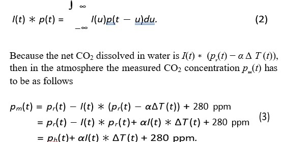
In the above equation p (t) is the human release of CO₂ to the atmosphere and ph (t) is the part of the human release, which stays in the atmosphere. More of the properties of convolution are presented in our book [6]. Next we have to calculate the human contributions in Eqs. (3). We are lucky that Hermann Harde [8-10], has fitted in an exponential form the estimated anthropogenic CO₂ release rate dpr(t)/dt, which includes the land use, too. In the fit the time interval was between 1850 and 2010. The result is given by

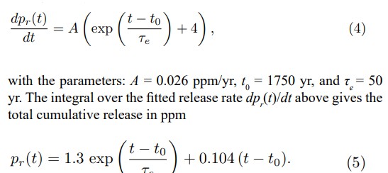
This agrees very well with the observation. Note that pr(t) goes directly to the atmosphere. The advantage of the above analytical form of pr(t) is that we can calculate an analytical expressionof the convolution I(t) ∗ pr(t), because pr(t) has exponential and linear terms. So, we can calculate pr(t) − I(t) ∗ pr(t) = ph(t) or the anthropogenic concentration, which stays in the atmosphere from the release pr(t). Note that I(t) ∗ pr(t) dissolves in water. Thus, the result is given by If dpr(t)/dt is a constant, then ph (t) = τ dpr (t) / dt, which is useful in the estimation of carbon sinks. In order to attain our final goal, i.e., to derive α and τ we have two possibilities. First we calculate the convolution α I (t) ∗ â??T (t) = pe(t). Now according to Eqs. (3) ph(t) + pe(t) + 280 ppm should be the measured CO2 concentration pm(t) (the smoothed Keeling curve) in the atmosphere. Thus, by comparing the calculated concentration with the measured one pm(t) we are able to derive τ and α. However, the computations of convolution integrals are a little problematic, because in convolution at a certain point requires measured data even 3τ earlier than this point. Convolution has a memory effect. The second possibility is to carry out the calculation backwards, i.e., the calculation of â??T comparing the calculated concentration with the measured one pm(t) we are able to derive τ and α. However, the computations of convolution integrals are a little problematic, because in convolution at a certain point requires measured data even 3τ earlier than this point. Convolution has a memory effect. The second possibility is to carry out the calculation backwards, i.e., the calculation of â??T 

Figure 1 shows the functions needed in computation: Human cumulative released pr(t) Eq. (5), pm(t) − 280 ppm i.e., about one year Fourier-smoothed Keeling curve, ph (t) Eq. (6) and finally pe(t) = pm(t) − 280 ppm − ph(t) [6,11]. Note that the human contribution ph(t) is small only about 12% of pr(t).

Experimental Derivation of The Response Time Τ and the Global Emission Strength α

Figure 2 shows five observed temperature anomalies â??Ta(t) according to Ole Humlum [12]. As you can recognize, these anomalies deviate quite a lot from each other, even 0.425°C. However, the overall temperature increase is clear and El Nin˜o,  too. The anomalies UAH MSU and RSS MSU oscillate more than the three others. Even those better three anomalies differ of the order of 0.15°C from each other. Now we are ready to derive α and τ so that the calculated temperature â??T (t) according to Eq. (7) explains the measured temperature â??Tm(t), which is the average of the anomalies â??Ta(t) + Ã¢??Tref . We carry out a nonlinear least square fit of the function â??T (t) to â??Tm(t). The extra fitting parameter â??Tref is the

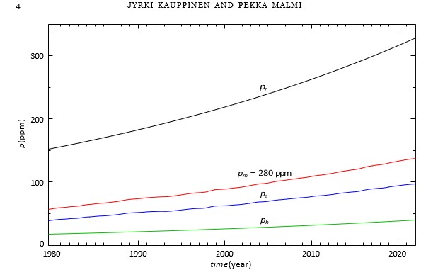
Figure 1: Human CO2 release pr(t) (black), measured pm(t) − 280 ppm (red), CO2 emitted by water pe(t) (blue) and human CO2 contribution to the atmosphere ph(t) (green)

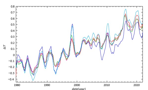
Figure 2: One year running averages of global monthly temperature anomalies normalised by comparing to the average value of 30 years from January 1979 to December 2008 [12]. UAH MSU (blue), RSS MSU (cyan), GISS (red), NCDC (magenta) and HadCRUT5 (green)

temperature, which we have to add to the anomalies so that they reach the level of the calculated â??T(t). Using the average of all the five anomalies smoothed by one year moving average in â??Tm(t) the fit gave α = 82.7 ppm/°C, τ = 7.43 yr and â??Tref = 0.801°C. This fit is the calibration of the thermometer. Most of the reported residence times are 5 − 10 years [13]. The final results are seen next in Figure. 3. We repeated the above fit using only three better measured temperature anomalies and their average. This fit resulted in α = 84.9 ppm/°C and τ = 6.30 yr.

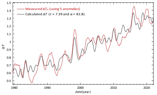
Figure 3: The red curve is the average of all the five anomalies in Figure. 2 added by ΔTref = 0.801°C. The black curve is calculated from Eq. (7) with α = 82.8 ppm/°C and τ = 7.39 yr.

Figure 4 shows the temperatures calculated using the above derived α and τ in the cases, where we used three and five measured temperature anomalies. This figure gives us a hint how much the used measured temperature anomalies affect the precision of the thermometer via the parameters α and τ . Even though the measured temperature anomalies are quite inaccurate, the maximum error of the calculated temperature is only 0.03°C. In figure 5 we have tested the accuracy of the method caused by possible errors in the measured pm(t). Two temperature curves are calculated using as pm(t) the Mauna Loa and the global CO₂ curves [14,15]. As you can see, differences are mainly well below 0.1°C. However, the errors of pm(t) dominate. Thus, according to Figures 4 and 5 we can conclude that the precision of our global thermometer is better than 0.1°C using only a single measured CO₂ curve. Of course, the accuracy can be improved using the average of many CO₂ observations and a longer smoothing time.

Causality: Temperature Is A Cause of Co2

According to our theory, the causality means that the temperature change â??T (t) produces the most CO₂ via the convolution pe(t) = αI(t) ∗ â??T (t). It is well known

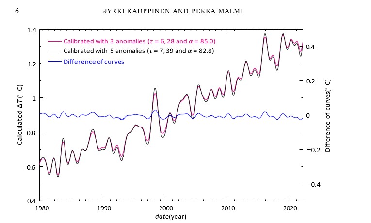
Figure 4: The temperatures calculated using the average of the temperature anomalies GISS, NCDC and HadCRUT5 with τ = 6.28 yr and α = 85.0 ppm/°C (purple) and the temperature anomalies GISS, NCDC, HadCRUT5, UAHMSU and RSSMSU with τ = 7.39 yr and α = 82.8 ppm/°C (black).

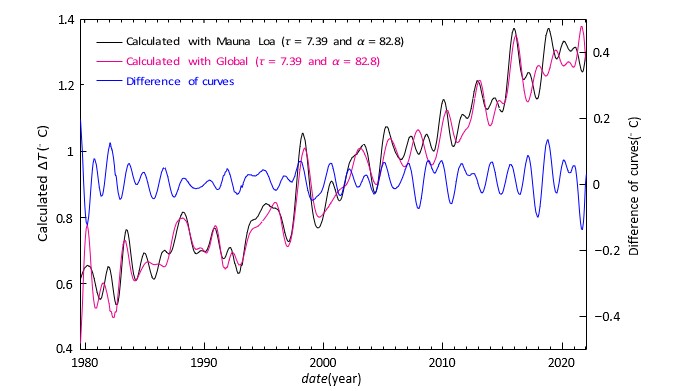
Figure 5: The temperatures calculated using the average of the temperature anomalies GISS, NCDC, HadCRUT5, UAHMSU, RSSMSU and the Mauna Loa CO₂ curve (black) and the global CO₂ curve (magenta).

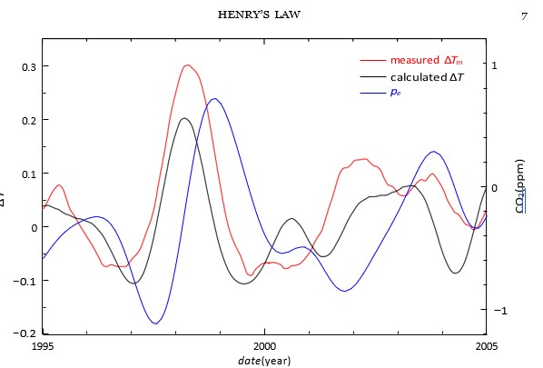
Figure 6: A detail of Figure. 3 around the El Ni˜no peak 1998 superimposed with the CO₂ curve pe (blue).

That effects never precede their causes. The causality is the basic property of the convolution by I(t), which is zero when t < 0. With the help of Figure. 6 we will demonstrate the causality using the measured signals in a real case.

Figure 6 shows the measured temperature â??Tm(t), the measured CO₂ concentration pe(t), and the calculated temperature â??T (t) around the El Nin˜o peak 1998. We have subtracted from the above curves a parabolic baseline in order to see better the El Nin˜o peaks. In this figure you can find that the measured â??Tm(t) and the calculated â??T (t) are very similar, but the measured CO₂ in pe (t) is delayed about one quarter its period. This is the proof that the temperature change causes the major CO₂ change, not vice versa. Ole Humlum has studied experimentally the same El Nino˜ peak and its delay [16]. Our results are in a very good agreement with those of Ole Humlum.

According to IPCC, the main cause of climate change is CO₂. Thus, using the climate sensitivity we can calculate the temperature peak from El Nin˜o CO₂ peak of about 1.8 ppm in Fig. 6. So, according to IPCC, the amplitude of the temperature peak should be about 0.24°C ln((420 + 1.8)/420)/ ln 2 = 0.00148°C. In addition, the peak has the further delay of about one month. This should be the amplitude of the observed or the calculated temperature peak in Fig. 6. However, the measured peak is about 0.37°C and the calculated one 0.32°C. The calculated peak is approximately τ/α times the derivative of pe(t). All strongest real temperature peaks are followed by lagged CO₂ peaks with a similar manneras the El Nin˜o peak. See also the figures of Ole Humlum [16]. The above calculation means that the method of IPCC to calculate temperature changes is completely wrong in magnitude, even if we use ten times higher sensitivity like IPCC. The most important thing is the fact that the IPCC method produces the temperature peak at a wrong position nearly one year later than the measured one. These are the strong proofs, that the causality used in IPCC reports is wrong. Thus, we have proven that merely the greenhouse effect cannot explain climate change.

Carbon Sinks

If the human release pr(t) and ph(t) go rapidly to zero, then after 3τ the global temperature has dropped about 0.03°C. This gives us a hint, how much we can affect the temperature using carbon sinks. The forests are good carbon sinks. We have land less than 29% of the area of Earth. About one third of land is coved by forests, which absorbs CO₂ about 15 Gtn/yr. In principle, we can double the area of forests, which lowers the temperature approximately 0.01°C.

Discussion

One very important advantage of the calculated â??T (t) is that it gives the temperature in the right and real scale, whose zero value is on the level, where CO₂ is 280 ppm.

As shown in Figure. 4, there is a clear need of the more accurate measurement of the global temperature. Carbon dioxide is an indicator of the global temperature. That is why we have proposed a new thermometer for the global temperature based on the Eq. (7). We can use every month measured CO₂ data pm(t) at Mauna Loa to calculate the points in pe(t) by subtracting the known human release ph(t) from pm(t). So, we can calculate a new temperature value every month but six months later, if we smooth pm(t) by one year moving average.

It is important to realize that Henry’s Law uses all the possible water surfaces: oceans, lakes, rivers, and even water drops in rainfall and on the leaves of trees. In addition, in the atmosphere all the gases obey Henry’s Law. However, we do not need to know in detail the ocean chemistry and the Henry’s Law constant, because we use measured global values of pm(t), pr(t), and â??Tm(t). These values included all the needed knowledge. In addition, we do not like to handle the problem locally like James R. Barrante, but instead we use global values [17]. The net CO₂ dissolved in water mainly in the oceans is I(t) ∗ (pr(t) − αâ??T (t)), which acidifies the oceans so that pH is decreasing. The calculated temperature â??T roughly consists of −11°C â??c + GH + GH(human), where â??c is a change of low cloud cover, GH is a greenhouse term of the extra CO₂ due to the warming of −11°C â??c, and GH(human) = 0.24°C ln((420 + ph (t))/420)/ ln 2 = 0.029°C in 2020. At last, we have to point out that τ and α derived in this paper are valid in a limited temperature range. Theoretically α depends on the temperature slightly exponentially. The study of this question requires more precise measured temperatures. On the other hand, we have the Keeling curve down to 1960 so we can calculate the temperature down to 1960, too. Around 1973 it was a quite strong El Nin˜o. We do not show this part of the temperature, because there is no good measured temperature for comparison.

Conclusion

In an equilibrium, Henry’s Law is very trivial and we do not need to calculate any convolutions. But, if the climate is out of the equilibrium, then we have to apply the unit impulse response via convolution in order to describe concentrations as a function of time. Right now, our climate is substantially out of balance, because of the big human CO₂ release and the change of low cloud cover. In this situation, we must use our theory to study climate change.

Nature convolves the true temperature â??T(t) by αI (t). The convolution is pe(t) the CO₂ concentration emitted to the atmosphere. According to Eq. (7), deconvolution back is very simple â??T (t) = (pe(t) + τdpe(t)/ dt)/α. In other words, in deconvolution we search for the temperature the convolution of which is pe(t). This is a very useful result, which we are able to use as a new thermometer for global temperature. The theory is exact, but only noise or errors in the measured â??Tm(t), pm(t), and ph(t) limit the accuracy of this method. Note that the method does not depend on the cause of the temperature change. The results of this work confirm our earlier studies about climate change [7,18- 20]. Since 1970, according to the observations, the changes of the low cloud cover have caused practically the observed temperature changes [18-21]. The low cloud cover has gradually decreased starting in 1975. The human contribution was about 0.01°C in 1980 and now it is close 0.03°C.

References

- Hartmann, D. L. (2015). Global physical climatology (Vol. 103). Newnes.
- Henry, W. (1803). III. Experiments on the quantity of gases absorbed by water, at different temperatures, and under different pressures. Philosophical Transactions of the Royal Society of London, (93), 29-274.
- Wikipedia contributors. Henry’s law — Wikipedia, the free encyclopedia, 2023. https://en.wikipedia.org/w/index. php?title=Henry%27s_law.
- Smith, F. L., & Harvey, A. H. (2007). Avoid common pitfalls when using Henry's law. Chemical engineering progress, 103(9), 33-39.
- Sander, R. (2015). Compilation of Henry's law constants (version 4.0) for water as solvent. Atmospheric Chemistry and Physics, 15(8), 4399-4981.
- Kauppinen, J., & Partanen, J. (2001). Fourier transforms in spectroscopy. John Wiley & Sons.
- Kauppinen, J., Heinonen, J. T., & Malmi, P. J. (2011). Major portions in climate change; physical approach. International Review of Physics, 5(5), 260-270.
- Harde, H. (2019).What humans contribute to atmospheric CO2: Comparison of carbon cycle models with observations. Earth Sciences, 8(3), 139-159.
- Le Quéré, C., Andrew, R. M., Friedlingstein, P., Sitch, S., Pongratz, J., Manning, A. C., ... & Zhu, D. (2018). Global carbon budget 2017. Earth System Science Data, 10(1), 405-448.
- Oak Ridge National Laboratory. Annual global fossil-fuel carbon emissions. https://cdiac.ess-dive.lbl.gov/trends/emis/ glo_2014.html.
- Kauppinen, J. K., Moffatt, D. J., Mantsch, H. H., & Cameron,D. G. (1982). Smoothing of spectral data in the Fourier domain. Applied optics, 21(10), 1866-1872.
- O. Humlum. https://www.climate4you.com/images/AllInOneQC1-2-3GlobalMonthlyTempSince1979. gif.
- L. Solomon. (2008).The deniers, pp. 82-83, 2008. https:// c3headlines.typepad.com/.a/6a010536b58035970c0120a5e5 07c9970c-pi.
- NOAA US Department of Commerce. Global monitoring laboratory - carbon cycle greenhouse gases. https://gml.noaa. gov/ccgg/trends/mlo.html.
- Global monitoring laboratory - carbon cycle greenhouse gases.
- Humlum, O., Stordahl, K., & Solheim, J. E. (2013). The phase relation between atmospheric carbon dioxide and global temperature. Global and Planetary Change, 100, 51-69.
- J. R. Barrante. https://climaterx.wordpress.com/2014/07/26/carbon-dioxide-and-henrys-law.
- Kauppinen, J., Heinonen, J., & Malmi, P. (2014). Influence of relative humidity and clouds on the global mean surface temperature. Energy & Environment, 25(2), 389-399.
- Kauppinen, J., & Malmi, P. (2018). Major feedback factors and effects of the cloud cover and the relative humidity on the climate. arXiv preprint arXiv:1812.11547.
- Kauppinen, J., & Malmi, P. (2019). No experimental evidence for the significant anthropogenic climate change. arXiv preprint arXiv:1907.00165.
- Düba l, H. R., & Vahrenholt, F. (2021). Radiative energy fluxvariation from 2001–2020. Atmosphere, 12(10), 1297.