Identification of Missing Data and Imputation in Vaccination Rates for an Ecological Study of the Southern Cone of South America in Four Countries

Introduction

In epidemiological studies with an ecological design, it is common practice to work with country-level data from secondary data sources. For this reason, a harmonization process is required to ensure the quality and completeness of the data, as a fundamental element of what is known as reproducible research. In general, data from secondary sources do not always contain completely complete data, and their quality is not always excellent. Part of the explanation for this weakness is due to the origin of the data that these portals then publish. Either the agencies themselves impute or report average data from past periods, or they simply disclose what they received, and the missing and/or anomalous data appear. Regardless of what ultimately happens when releasing the data, it must be ensured that the harmonization process is transparent when accessing the repositories, ensuring reproducibility [1-5]. This section presents the different stages that allow for establishing a workflow, as detailed below:

STAGE 1 - Data harmonization (prior to data processing) and project preparation in the software to be used.

STAGE 2 - Implementation of the information system with a graphical uinterface for downloading data from secondary data sources

STAGE 3 - Exploratory analysis and variable selection.

STAGE 4 - Visualization of missing data.

STAGE 5 - Imputation of missing data.

STAGE 6 - Interactive visualization (R Shiny).

 The life cycle of this work consists of a first advance presented in August 2024 with an extended summary for the XVII Semana Internacional de la Estadística y la Probabilidad, de la Facultad de Ciencias Fisico Matemáticas at Benemérita Universidad Autónoma de Puebla, with preprint number https://doi. org/10.5281/zenodo.13763282; It is subsequently supplemented with the almost completed work prior to the preparation of this document, presented at the conference Jornadas de Estadística Octubre de 2024 in Montevideo, Uruguay, available en https:// doi.org/10. 5281/zenodo.14652623. Finally, the work was uploaded as a preprint on the Scielo preprint platform, available at the following link: https://preprints.scielo.org/index.php/ scielo/preprint/view/12147/version/ 12794. To ensure the reproducibility of the results of the analysis performed, the code and data used are available in a public repository on the OSF platform which can be accessed through https://osf.io/6r3ew/. The document is structured as follows: A Material section in 2.1 on page 3, followed by the methods appearing in the 2.2 section  of page 4,finally proposing some conclusions from what has been found so far and possible methodological steps to follow,in the 3 section of page 18.

Materials & Methods

Material

In this section, given the nature of the work, which consists of using secondary data sources, the available data are presented, where the number of variables, their definitions and where they are extracted from are considered, as part of the flowchart presented in the previous section.

Vaccine Block

All the vaccines initially considered in this study are listed below. It should be noted that the information used is corresponding to 20 years from 4 countries (Argentina, Chile, Paraguay, Uruguay), so the vaccine block was originally supposed to have 1,520 records (19*20*4). However, there are 1,360 missing records; therefore, from this block of 19, taking into account the lack of information for this study, only 7 immunopreventable pathologies will be considered through the corresponding rates, and from which a block called RVB, for Reduced Vaccine Block, is created.

HEPB3: Hepatitis B; third dose

HIB3: Haemophilus influenzae type B; third dose

POL3: Polio; third dose

DPT1: Diphtheria, Pertussis, Tetanus; first dose

MCV1: Measles, first dose

MCV2: Sarampion; second dose

DPT3: Difteria, Pertusis, Tétanus; third dose

Methodology

The methodology used after data harmonization consists of 3-dimensional analysis.

• Analysis of quality data and missing data (see section 2.2.1).
• Imputation of missing data (see section 2.2.5).
• Statistical analysis of the information: harmonized data and imputed using different methodological approaches.

Missing Data for Vaccine Block

Structured data is loaded in long format, that is, there is a data table with 80 observations corresponding to the 4 countries studied in the time period 2000 to 2019. In this part of the data preparation, the R software is used with libraries such as psych, the Rstudio interface, with readxls and knitr [[6-10]. It is important to remember that in section 2 it was stated that we would work with the Reduced Vaccine Block (hereafter referred to as RVB). The reduced vaccine block and country and year identifiers are created for the analysis. Below are the first 6 records of the table for 10 years, that is, back 10 years to 2019.

Although the analysis is carried out for the last 10 years and for the 20 years, due to length issues only the results for 20 years are presented.

Analysis of Vaccine Blocks Over the Past 20 Years (2000-2019)

In this section, we analyze data from the 20 years of analysis and visualize missing data. The naniar library is used to identify missing data patterns [11].

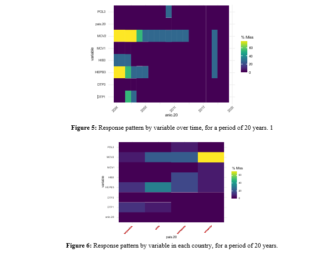
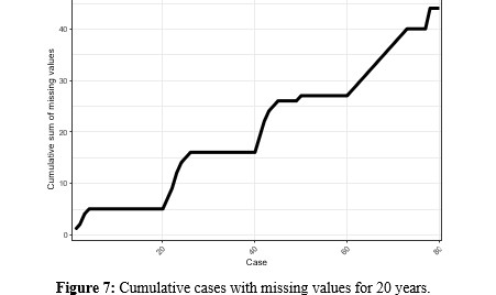
From Figure 1 it can be said that for the 20-year period, again the MCV2 vaccine is the one with the greatest number of missing values. In Figure 2, on the one hand, you can see the non-response pattern by country. The MCV2 vaccine has almost 30. On the other hand, you can see the observations with values above 100%, with MCV1 being the vaccine with the most anomalous values.

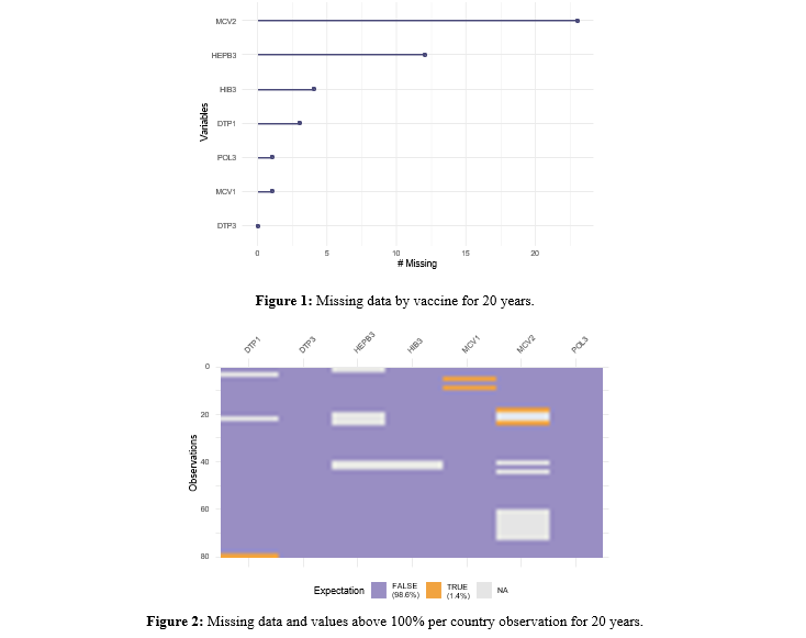
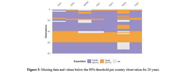
To investigate whether there is a pattern for observations below the 90% threshold, Figure 3 is created, which shows that again Paraguay, in the 20 years, is the country with insufficientimmunization and only for MCV2, Argentina and Chile show low immunization.

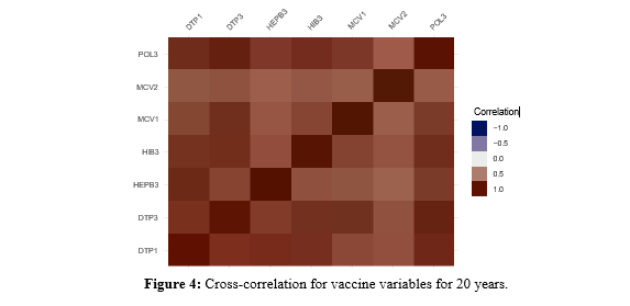
As Figure 4 shows, the correlations between vaccines are all still positive.

Exploring Other Patterns for a 20-Year Period

For the period from 2010 to 2019, Uruguay is the country with the most missing values occurring over the 10 years.

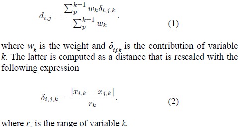
When expanding the time window and considering the period from 2000 to 2019 (Figure 7), Argentina is the country with the fewest missing values, followed by Chile and Paraguay, which concentrate the missing data in the first years. Uruguay shows that it only has complete values in 5 years, this being for the latter part of the period, and where the vaccine with the most missing values, as seen in previous sections, is MCV2.

Based on what is observed in the different figures, it is noteworthy that:

• In general, there are more missing values when considering the 20-year period, concentrated in (2010−2019).
• Paraguay is the country with the lowest vaccination rate for most vaccines, below 90 %.
• The rates show a positive linear correlation.

• Rates above this value must be truncated at 100; in this case, they are MCV1, MCV2, and DTP1.
• MCV2 must be imputed for several years in Uruguay, and for that vaccine, Argentina has almost complete information.
• Imputation must be made for the last two years in Uruguay in the variables HEPB3, HIB3, MCV1, MCV2, while the same imputation must be done in Chile at the beginning of the period.
• DTP3, MCV1, and POL3 have no missing data, except for one year in Paraguay

Imputation Proposals

Some of the proposed methods for handling missing data are presented below:

Hotdeck method Hotdeck, stratified by country. This means that the imputation of missing data for each variable depends only on the values for that variable and for that country, and does not consider data from other countries. The imputation mechanism consists of detecting when one or more missing data items are present for a given year and country and receiving a donor, which is the last available data item. The Hotdeck function belongs to the VIM library, [12].

Univariate method kNN. The kNN function of the VIM library performs a k-nearest neighbor imputation based on a variation of the Gower distance (Gower 1971) for numerical, categorical, ordered, and semicontinuous variables. In this case, a radius of size k is set, which allows for considering observations that cluster according to the distances between each row (remembering that these are each year in a country). Since the results are very similar to those found for Hotdeck, this imputation version is not considered. [12]. Like the hotdeck method, the k nearest neighbor method is based on the observation of donor values, that is, it uses an aggregation of the k closest values as the imputed value, and the type of aggregation depends on the type of variable. The calculation of the distance to define the nearest neighbors is based on an extension of the Gower distance, the distance between two observations being the weighted average of the contributions of each variable, where the weight should represent the importance of the variable, therefore, the distance between the i-th and j-th observation can be defined as 

Multivariate method with the Amelia function and library. This method uses an EM (expectationmaximization) and bootstrap algorithm. It also allows you to work with more than one imputed data table per block and also consider the data as if they were panel data (which is the case). Since this is a multivariate method, considering only the matrix with missing data per block is not the same as considering an entire block. [13-16]. As a result of the imputation, the solution of an EM (expectation- maximization) and bootstrap algorithm, a series of imputed tables are obtained, which must then be averaged. A feature of this method is that it assumes a multivariate normal distribution.

• The assumptions for the multivariate method are:
• The imputation model on which the algorithm is based assumes that the complete data (i.e., both observed and unobserved) have a multivariate Gaussian distribution.
• D ∼ Nk(µ,σ2), where D = Dobser,Dfalt
• The algorithm also assumes that it only observes Dobs, and not D, and that missing data have a MAR-type mechanism. This is equivalent to assuming that the pattern of missing data only depends on the observed data Dobs
• If M is the missingness matrix, with cells mij = 1 if it is missing data or 0 if it is observed data

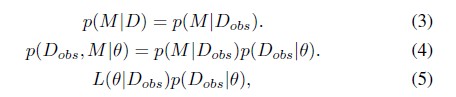
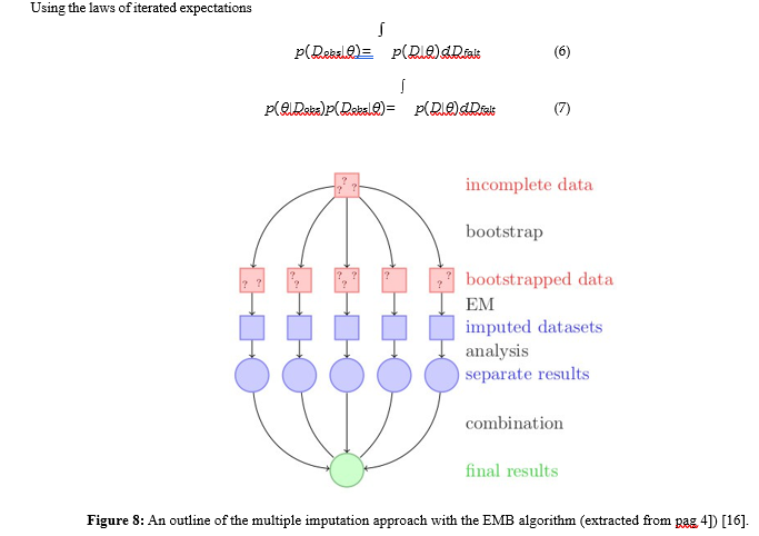
Using the laws of iterated expectations

• • The EMB algorithm combines the classical EM algorithm with a bootstrap approach to draw samples from the posterior distribution
  • For each run, a bootstrap sample is drawn to simulate the uncertainty of the estimate, and then the EM algorithm is run to find the posterior mode of the sampled data, [15].
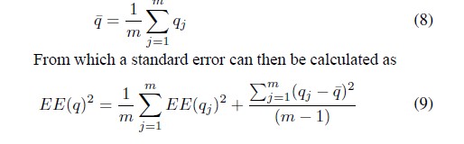
  • If we are interested in estimating the quantity q, a mean, regression coefficient, etc., what we can do is work with m imputed data sets and obtain an average of the m estimates made separately

   Imputation for Vaccines
Based on the study of missing data, the possible imputation mechanisms are:
•    Scenario 1: If missing in t, impute by the mean of t − 1;t + 1 if possible.
•    Scenario 2: Impute by the period mean.
•    Scenario 3: Test an imputation mechanism such as Missing Completely at Random (MCAR), Missing at Random (MAR), or Missing not at Random (MNAR). In particular, decide whether to proceed with univariate or multivariate imputation (using the methods presented in the ?? section) and also consider an imputation mechanism that takes into account the fact that these are panel data.
The RVB is considered

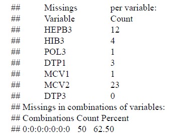
Figure 9 shows, on the one hand, the proportion of missing data (right-hand side) and, on the other, the different combinations of variables (vaccines in this case) with missing data and their proportion in the total (left-hand side of the figure). To better understand the latter, some cases are detailed. There are observations (country-year) that do not have any missing values, so the first row of the figure on the left is filled with light blue rectangles. This is also observed in most observations, as the bar at the end of the row is the largest. Next comes the row where the only pink rectangle is in the variable MCV2, indicating that there are observations where the only missing value is in the variable MCV2. At the other extreme, the last row shows that the variables HEPB3, HIB3, MCV1 and MCV2 are colored pink, which means that there are observations with missing data in those four variables, but these are the cases that are least observed since the bar at the end is the smallest.

The number of missing values for each of the 7 vaccines is shown below. As seen in the section on missing vaccine values, MCV2 has the most (23 observations).

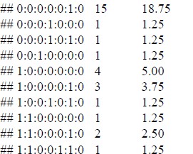
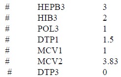
This last table reflects what is shown in the previous figure but adds information on how many observations have missing values for a given set of vaccines. There are 50 observations (country- year) that have no missing values in any observation. This is followed by 15 observations that only have missing values in column 8. Considering the previous figure, it is clear that this corresponds to the MCV2 vaccine. The average of consecutive data with missing values is shown here for each variable. In HEPB3, there are, on average, three consecutive observations with no data.

Imputation by Hotdeck Method for RVB

From the data, where the missing values have already been identified, after applying the Hotdeck method the results are:

                                                        Table 1: Values imputed by Hotdeck method.

Imputation by kNN Method

Imputation is performed using the kNN method, setting a radius of 5 for the group size, i.e., considering the distances between the four nearest neighbors. Like the hot-deck method, the k nearest neighbor method is based on the observation of donor values; that is, it uses an aggregation of the k closest values as the imputed value. Again, in Table 2, some statistics for the vaccine variables can be seen before and after the imputation process, but this time using kNN, where it is again observed that, in general, the means do not change substantially.

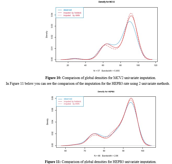
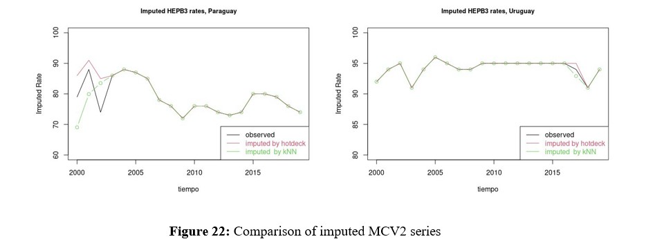
In Figure 10 below you can see the comparison of the imputation for the MCV2 rate using 2 univariate methods.

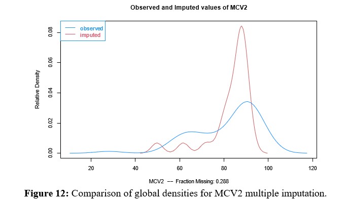
Multivariate Imputation for MCV2

Before performing the multivariate imputation procedure with the Amelia library, the restriction must be set to limit the rates to the range [0,100]. Figure 12 shows the observed (blue) and estimated (red) densities for the variable MCV2, which had the largest amount of data to impute. Then, graphs of the observed (black) and imputed data values, along with their confidence intervals (red), are shown for each of the four countries for the aforementioned variable, MCV2.

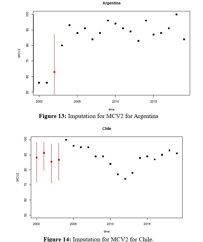
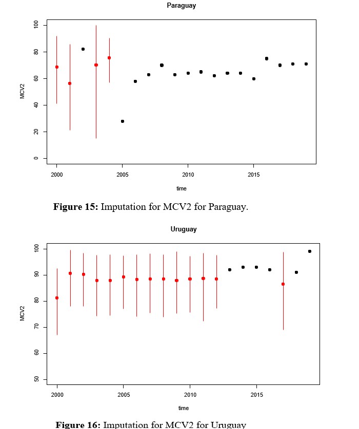
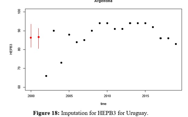
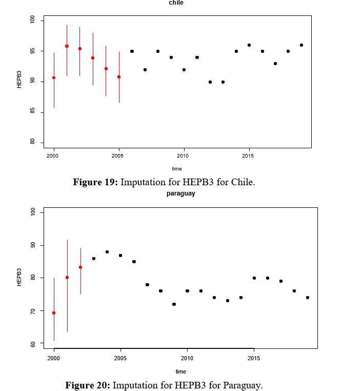
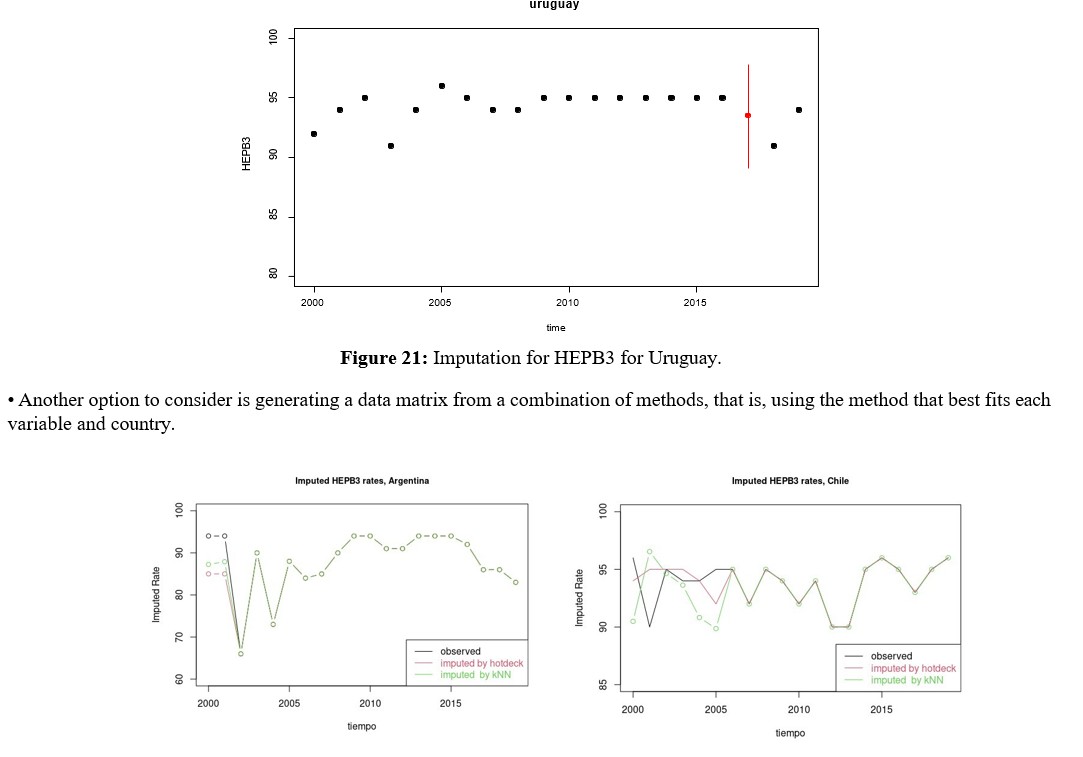
Remembering that the vaccination rates that make up the RVB block can be viewed as panel data, it is important to see the result produced by the multivariate imputation, which is why the imputed values for each country are shown instead of the densities, but assuming that the 7 rates are a multivariate random variable of dimension p = 7 and whose structure is incorporated over time. For this purpose, when there is an imputation, a red segment appears that not only represents when there is an imputed value, but also a bound on the imputation error through a confidence interval, as shown in figures 13, 14, 15.

Finally, the observed (blue) and estimated (red) densities for the remaining 6 imputed variables of the vaccine block are shown.

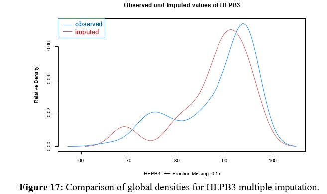
Multivariate Imputation for HEPB3

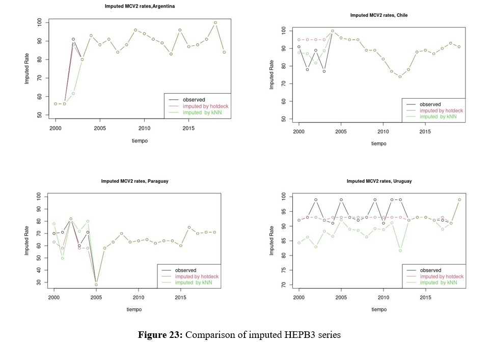
Since HEPB3 is the second vaccine, along with MCV2, with the greatest amount of missing data, multivariate imputation of the same is evaluated in this section. In this case, it can be seen in Figure 17 that the density of the imputed variable remains bimodal with a shift towards the center, where the weight of Paraguay can be seen. Before deciding which of the methods to work with, comparisons of the rates imputed by Hotdeck and kNN are presented in figures 22 and 23 for MCV2 and HEPB3 respectively. These in turn must be compared with the Figures 13, 14, 15 y 16 para MCV2 y 18, 19, 20 y 21 for HEPB3, which show multivariate imputation.

Conclusion

Conclusions and Next Steps with the Imputation of RVB Taking into account the densities of the univariate imputations, which appear in figures 10 and 11 made with the Hotdeck and kNN methods, it is found that:

• For the case of HEPB3 the fit is quite good, while for MCV2 (variable with the greatest amount of missing data) both methods tend to accentuate the 2 modes of the density.
• When evaluating the performance of the multivariate method, Figures 13 and 16 show that the fit between the observed and imputed data is lower. This is especially true for the case of MCV2, which tends to globally concentrate the data in a range of [80,100]. If we evaluate how it is at the country level for the case of MCV2, given that they are at the extremes of the series and at the beginning of it for Chile and Paraguay, the imputed values fluctuate with great variability in the range [70,100] and where Uruguay has an imputed value on average that barely varies in the first 10 years.
• On the other hand, the values imputed using the multivariate method are positioned in each series, breaking the trend with which it has been fluctuating for some rates, such is the case for Argentina for HEPB3.

• • For the case of HEPB3, since the amount of missing data is smaller, the local variability (by country) also decreases and where the aspect to be rescued is that at the extremes of the series at the beginning of the period, in the imputation for Paraguay the rate grows, while in Chile a decrease in the rate is seen.

The results for the multivariate imputation mechanism may be due to these possible causes:

• The method relies on the assumption of multinormality of the variables.
• The number of observations (n = 20) per country is insufficient.
• Since in this case the variables to be imputed are percentages, they clearly cannot conform to a multinormal distribution, unless a transformation is performed.
• For these reasons, and taking into account the comparisons arising from the imputed rates, the following strategy is considered:
• Begin imputing using the kNN mechanism, which appears to generate the fewest fluctuations over the period.
• Then impute using Hotdeck and Amelia.
• Finally, compare the cluster results obtained using each of the three proposed methods.

Declaration of Funding

 Declaration of funding sources and conflict of interest. The authors declare that they had no external funding source for this research.

Authors Contribution

Ramón Álvarez-Vaz Conceptualization, Formal analysis, Data curation, Investigation Methodology, Project administration, Software, Validation, Visualization, Writing the original draft, and Writing the article. Silvia Rodríguez Collazo Conceptualization, Investigation, validation, visualization, and writing the original draft. Mauro Loprete Data curation, Methodology, Software, Validation, and Visualization.

Acknowledgements

To the entire team of Faculty of Economic and Administration Sciences, University of the Republic that faithfully collaborated with the investigation. Thanks also to Mikaela Lezcano for her feedback on the project and her data curation work in the early stages of the project.

References

16. Honaker, J., King, G., & Blackwell, M. (2011). Amelia II: A program for missing data. Journal of statistical software, 45, 1-47.

References

- Peng, R. D. (2009). Reproducible research and biostatistics. Biostatistics, 10(3), 405-408.
- Gandrud, C. (2018). Reproducible research with R and R studio. Chapman and Hall/CRC.
- Glennie, R. (2021). Reproducible Research with R and RStudio by Christopher Gandrud.
- Kohrs, F. E., Auer, S., Bannach-Brown, A., Fiedler, S., Haven, T. L., Heise, V., ... & Weissgerber, T. L. (2023). Eleven strategies for making reproducible research and open science training the norm at research institutions. Elife, 12, e89736.
- R Core Team 2022. R: A Language and Environment for Statistical Computing, R Foundation for Statistical Computing, Vienna, Austria. https://www.R-project.org/
- Revelle, W. 2022 . psych: Procedures for Psychological, Psychometric, and Personality Research, Northwestern University, Evanston, Illinois. R package version 2.2.9. https://CRAN.R-project.org/package=psych
- RStudio Team 2020 . RStudio: Integrated Development Environment for R, RStudio, PBC., Boston, MA. http:// www.rstudio.com/
- Bryan, H. W. (2022). J. readxl: Read Excel Files. R package version 1.3, 1.
- Xie, Y. (2017). Dynamic Documents with R and knitr. Chapman and Hall/CRC. ISBN 978-1498716963. https://yihui.org/knitr/
- Tierney, N., Cook, D., McBain, M. Fay, C. 2021 . naniar: Data Structures, Summaries, and Visualisations for Missing Data. R package version 0.6.1. https://CRAN.R-project. org/package=naniar
- Kowarik, A., & Templ, M. (2016). Imputation with the R Package VIM. Journal of statistical software, 74, 1-16.
- Dempster, A. (1977). Maximum likelihood estimation from incomplete data via the EM algorithm. Journal of the Royal Statistical Society, 39, 1-38.
- King, G., Tomz, M., & Wittenberg, J. (2000). Making the most of statistical analyses: Improving interpretation and presentation. American journal of political science, 347- 361.
- Honaker, J., & King, G. (2010). What to do about missing values in timeâ?ÂÂseries crossâ?ÂÂsection data. American journal of political science, 54(2), 561-581