
Annals of Civil Engineering and Management(ACEM)
ISSN: 3065-9779 | DOI: 10.33140/ACEM


Research Article - (2025) Volume 2, Issue 2
Hydrology & AT Math
Received Date: Jun 07, 2025 / Accepted Date: Jul 16, 2025 / Published Date: Jul 24, 2025
Copyright: ©©2025 Paul T E Cusack. This is an open-access article distributed under the terms of the Creative Commons Attribution License, which permits unrestricted use, distribution, and reproduction in any medium, provided the original author and source are credited.
Citation: Cusack, P. T. E. (2025). Hydrology & AT Math. Ann Civ Eng Manag, 2(2), 01-04.
Abstract
In this paper, we put some Basic Hydrology Equations on a mathematical footing using our knowledge of AT Math.
Introduction
A Hydrologist claims that the Hydrologic Cycle is not an exact science. However, in this paper, we show that it is an exact science. It follows AT Math [1].
P- R - ET =0
P = Precipitation
R = Runoff
ET Evapotranspiration
t²- t -1 = 0
It-(Q/A) ·t-ET = ΔS
I = Precipitation
Intensity
Q = River Volume
A = Drainage area
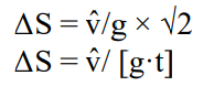
ΔS = Storage
ΔS = 2t-1
ΔS = ΔSs + ΔSg
ΔSs = Change in Storage in surface water
ΔSg = Change in Storage in groundwater
(1/t) (1/t) (t-e1)
T = Tensor from Relativity = Period T = 1/freq = 1/t = E
R = P-A
(Q/A) ·t = t² - A
t² - t - 1 = 0
A = 1 A = F + ΔSs
ΔSs √P = ΔSs t
Where P = It
t = π
t²-t-1 = 57.29° = 1 rad = 100%
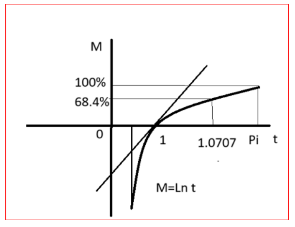
Figure 1: Rain Fall Intensity where 100% = t = Pi
Ober the long-term t = 161.8 or 161.8%
Hydrograph
Area Mt when M < 0
M = Ln t = Ln 1/2 = -0.693
0.15335(1/2) (1/2) = 0.767
1/Area = 0.0383375
GMPE = 1/sin θ = -1.25
θ=53.13 [=] dimensionless
0.684(0.5313) = 3634
1-0.3634 = 63652/π = 1/t = E
0.0383375/ (Ln 1/2) = 2.65≈SF
I = 3
t = √3
√3²-√3-1 = -2.67 = SF
d(mm) = 190 √D
Where D = duration
d = 190 √3 = 57≈57.29° = 1
π²-π-1 = 57.29 = 1 rad
IDF curve
I = 0.396 @t = 180 = 3(60) =3 Hrs
t = I = 190-39.6 =150.4 = 1/G = 1/E = t
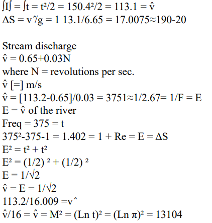
=1+31
=1+p#
In the following figure, imagine that one of the GMP s is perpendicular to the parge since the flow in a conduit is a parabola in perpendicular directions
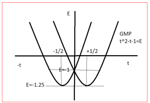
Figure 2: Stream Velocity Profiles
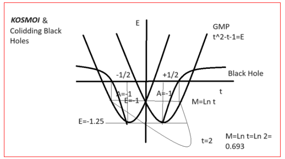
Figure 3: Rainfall Intensity and Stream Velocity profile. Critical Point is where t = 1/2 = 1.5 hrs
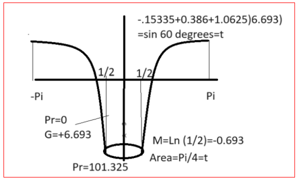
Figure 4
t² - t - 1 = E
1.5² - 1.5 - 1 = -0.25
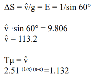
Triangle Weir:
Q = 1.42 tan (θ/2) H1.5 (SI)
Q = √2tan (π/2) H1.5
tan (π/2) = 57.518≈57.29 = E
Q = E ²Ht
Q/A = 1 = 2H1.5
1/2 = 1.5 Ln H
H = 1.3956≈1.4 = 1 + Re = ΔS
H = 1.132/9.806 = 11544 = 1/sin 60 = E when s = t
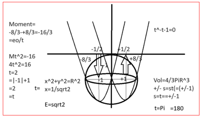
Figure 5
References
1. Verma, S., Engineering Hydrology. Fundamentals and Applications. Water Resources Engineering Vol II. Bolton Ontario, Amazon. (?)