Effect of Inflation Rate on the Agricultural and Manufacturing Sector in Nigeria (1990-2021)

Introduction

Inflation is a general increase in the prices of goods and services in an economy. When the general price level rises, each unit of currency buys fewer goods and services; consequently, inflation corresponds to a reduction in the purchasing power of money [1]. The common measure of inflation is the inflation rate; the annualized percentage change in a general price index. At global level as reported by Commodity Research Bureau (2009), the overall and food inflation rates stand at 16.5 and 30.2 percent respectively by November, 2007. Its effect particularly on agricultural products cannot be over emphasized as economists argued that it is the less productivity in agriculture sector and “so called” shortage of goods and services used in the production of agriculture sector that are considered responsible for inflation. This is made worst by the rise in prices in economy resulting from supply shocks of specific food items and to oil market in the world. The consequence of higher food inflation has caused households to make reductions in certain areas of food consumption resulting to malnutrition.

Nigeria’s inflation rate surged to a 65-month high of 18.6% in June 2022 from 17.71% recorded in the previous month, representing the fifth consecutive monthly rise in the rate of inflation. The last time the inflation rate in Nigeria touched the 18.6% ceiling was January 2017, when it stood at 18.72% [2]. On a month-on-month basis, the inflation rate increased to 1.82% in June 2022, this is 0.03% higher than the rate recorded in May 2022 (1.78%). Food inflation rose to 20.6% in June 2022 from 19.5% recorded in May 2022, while core inflation increased to 15.75% from 14.9% in the previous month. The uptick in the inflation rate is largely due to the surge in energy prices, which affected transportation costs across the country, and by extension rise in food prices .

In the manufacturing sector, The Food and Non-Alcoholic Beverages sub index is by far the most important, accounting for nearly 50% of total weight. Compared to the previous month, consumer prices increased 1.82%, after a 1.78% rise in May (NBS, 2022). The most important categories in the CPI are Food and Non-Alcoholic Beverages (51.8% of total weight); Housing, Water, Electricity, Gas and Other Fuel (16.7%) and Clothing and Footwear (7.7%). Transports account for 6.5%of total index and Furnishings and Household Equipment Maintenance for 5 %. Education represents 3.9% of total weight, Miscellaneous Goods and Services 1.7% and. Alcoholic Beverages, Tobacco and Kola account for 1.1% of total index.

Nigeria’s annual inflation rate accelerated for the third straight month to 16.82% in April of 2022, from 15.92% in March. It was the steepest inflation rate since last August, amid widespread increases across all divisions on the back of surging global commodity prices. Main upward pressure came from prices of food & non-alcoholic beverages (18.37% vs 17.20% in March), by far the most relevant in the CPI basket, in line with prices of imported food (17.66% vs 17.56%). Like most African countries, Nigeria is grappling with rising prices of food, as the continent is still largely dependent on agricultural imports, especially grains. Also, soaring diesel prices and the ongoing dollar shortage contributed to the upward trend in inflation. The annual core inflation rate, which excludes the prices of agricultural produce, rose to a five-year high of 14.18% in April of 2022, from 13.91% in the prior month. On a monthly basis, consumer prices advanced by 1.76%, the most since last December [3].

In Nigeria, several researchers have reported that increase in the prices of agricultural commodities are due to inflation as such, making it a macroeconomic problem. The consequences are major economic distortions, instability in price levels which has caused dissatisfaction results of the agricultural sector, increasing poverty level and discouraging investors from investing in the agricultural sector . The results arrived at by Taiwo and Anthony (2011) suggests that inflation rate has a negative impact on the performance of the Nigerian economy. Considering the contributions of the manufacturing sector to the country’s GDP. Moreover, statistics has confirmed the low and decreasing contribution of manufacturing sector under study to the economy’s GDP. In the same vein, Rasheed (2020) investigated the productivity in the Nigerian manufacturing subsector using cointegration technique and an error correction model. The study indicates the presence of a long-run equilibrium relationship index for manufacturing production, determinants of productivity, economic growth, interest rate spread, bank credit to the manufacturing subsector, inflation rates, foreign direct investment, exchange rate and employment rate. The performances of these sectors are still low in the area of large-scale production. Since inflation is significant and having an increasing trend, there should be an increase in productivity, strong manufacturing base and large-scale agriculture (following the law of supply; increase in price of goods will lead to increase in quantity supplied). But both sectors due to their performance trends are having decreasing productivity. However, most research works have not studied the effect of inflation on specific products produced by some manufacturing firms i.e. the domestic manufactured goods of some specific product classification, and on the other hand specific produce or raw materials produced in the agricultural sector meant for further production of finished goods. Also, it is necessary to determine the extent at which inflation affects manufacturing inputs which are imported for production purposes. This is very important to do as this research work will be filling the above gaps.

Research Objectives

The main objective of this study is to examine the Effect of Inflation Rate on the Agricultural and Manufacturing Sector in Nigeria. Specifically, it sees to;

• Examine the effect of inflation rate on domestic manufactured goods.

• Evaluate the effect of inflation rate on agricultural domestic raw inputs.

• Evaluate the extent at which inflation rate affect the manufacturing import inputs.

Research Hypotheses

H01: There is no significant relationship between inflation rate and domestic manufactured goods.

H02: There is no significant relationship between inflation rate and agricultural domestic raw inputs.

H03: There is no significant relationship between inflation rate and manufacturing import inputs H1: There is a significant relationship between inflation rate and manufacturing import inputs.

Literature Review

International Production Theory

International production deals with production of goods and services in international locations and markets. It involves management process which has to take into consideration local production market (labour and capital) and international customer necessities. The international production encompasses vertical production chains extended across the countries in the region as well as distribution networks throughout the world. The major actors are corporate firms belonging to the machinery industries, including general machinery, electrical machinery, transport equipment, and precision machinery though some firms in other industries, such as textiles and garment, also develop the network. Theorists stated that International production is value adding activity owned or controlled, and organized by a firm outside its national boundaries . General theory of international production proposed by John Dunning first advocated in the late 1970s, has generated considerable discussion. This work thoughtfully reassesses the paradigm, and extends the analysis to Policy autonomy, their own official history of capital. Dunning's eclectic paradigm (OLI) has been the most influential framework for empirical investigation of determinants of foreign direct investment.

The Conservation Model

The conservation model of agricultural development evolved from the advances in crop and livestock husbandry associated with the English agricultural revolution and the concepts of soil exhaustion suggested by the early German chemists and soil scientists. The conservation model emphasized the evolution of a sequence of increasingly complex land and labour-intensive cropping system, the production and use of organic manures and labour-intensive capital formation in the form of physical facilities to more effectively use land and water resources. This model was the only approaches to intensification of agricultural production that was available to most of the world’s farmers. Agricultural development within the ambit of the conservation model, clearly was capable in many areas of the world of sustaining rate of growth in agricultural production around 1.0% per year over relatively long periods of time. This rate is not compatible with modern rates of growth in the demand for agricultural output which typically fall between 3-5% in the developing countries [4].

Methodology

Since the purpose of this research paper is to gain a better insight into the effect of inflation rate on agricultural and manufacturing sectors in Nigeria and the effects of various independent variables on the dependent variables. Manufacturing Value Added (MVA), whose some of its components are FOOD, TEXTILE, and LEATHER; Agricultural Value Added (AVA), whose some of its components are CROP PRODUCTION, LIVESTOCKS, and FISHING are the dependent variables, while Inflation rate (INF), credit to private sector (PRIVATECREDIT), manufacturing capacity utilization (MCAPUTIL), foreign direct investment (FDI), credit to agriculture (AGRICCREDIT), agriculture equipment (AGRICEQUIP)and Exchange rate (EXCH) as independent variables. Descriptive research was adopted to obtain necessary data for the study. In carrying out this paper work on effects of inflation rate fluctuations on agricultural and manufacturing sector in Nigeria, we develop a compact form of our model as follows:

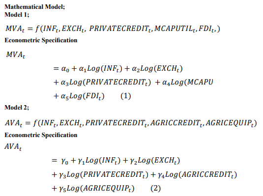
Model 1; Effect of Inflation rate on Manufacturing output

Model 2; Effect of Inflation rate on Agricultural output

Where; INFt denote the inflation rate at time t,

EXCHt denote the exchange rate at time t,

MVAt  denote the manufacturing value added i.e. manufacturing sector’ productivity as a % to GDP growth rate,

AVAt denote the agricultural value added at time t,

PRIVATECREDITt denotes credit to private sector at time t,

AGRICCREDITt denotes credit to agricultural sector at time t,

AGRICEQUIPt denotes agricultural equipment at time t,

FDIt denotes foreign direct investment at time t,

MCAPUTILt denotes manufacturing capital utilization at time t, 

α₁ and γ₁ are the slopes of the lag values of both the manufacturing sector and agricultural sector α₀ and γ₀ are the intercepts of the mathematical models,

While μt is the residual term which capture factors influencing the dependent variables which are not included in the model.

Estimation Techniques

This research work makes use of econometric approach in estimating the effects of inflation rate fluctuations on agricultural and manufacturing sector in Nigeria. The empirical analysis is being limited to the period between 1975 and 2020 due to the large number of years involved. Information and data needed for the study will be gathered from existing literature and from relevant government agencies such as the Central Bank of Nigeria (CBN), and international agency such as the World Data Index (WDI). The study utilized the Unit Root Test to check the stationarity or non-stationarity of the individual variable; after which the Auto Regressive Distributed Lag (ARDL) is the chosen estimation technique due to the nature of the variables, due to the result gotten from the unit root test, whereby some variables were stationary at levels I(0), while some were stationary at first difference I(1). ARDL is a suitable estimation technique when variables are at order 0 and order 1 only. It is important to know that ARDL will not be suitable to use when variables are at order 2. ARDL approach is appropriate for generating short run and long run elasticities for a small sample size at the same time.

Discussion of Findings

This section includes descriptive statistics on manufacturing GDP, agricultural output, interest rate, and exchange rate. It's a numerical description of the characteristics of the various variables that will be used and analyzed in the following sections. The data summary is shown below.

       Table 1: Summary of the descriptive statistics of manufacturing GDP, agricultural output, and all independent variables.

Researcher’s computation using EViews 9

The mean, median, minimum and maximum values, kurtoisis, skewness, and Jacque-bera for both the dependent and independent variables are shown in Table 4.1. The mean is a single value that reflects the centre of the series or the average value seen in the series. It is used to describe a sample. The FDI have a mean value of 0.067, which is the lowest among the series, while credit to agricultural sector has the highest mean value of 13.482. Like the mean, the median is a measure of central tendency that shows the value in the middle of the series that separates the higher and lower values. It's the number that splits a series in half.

The minimum and maximum values are the highest and lowest values in each time series, and the mean values of all series are within the boundaries of their minimum and maximum values. The standard deviation is the following statistics; it is a measure of the series' dispersion from its mean values. A high standard deviation indicates that the values in the series tend to be near to the series mean, whereas a low number indicates that the values are spread out over a broad range from the mean. A standard deviation number near to zero implies that the values are close to the mean, whereas a high or low value suggests that the values are above or below the mean. The standard deviation of all the variables is large, which is very far to zero; this observation shows that the values of all the variables have a wider range around their mean value.

Skewness informs the distribution features of the series; it measures the direction as well as the degree of asymmetry. A normal distribution is a symmetric distribution with a value of zero, a negative value of skewness indicates that the distribution is skewed to the left i.e. left-tailed in which case the mean is less than the median. The skewness values of agricultural output, credit to agricultural sector, manufacturing capacity utilization, foreign direct investment, exchange rate, crop, fishing, food, livestock, textile, and agricultural equipment is negative which means it is distribution have a left-tail, and the rest of the series are exhibiting the features of a right-tailed distribution as they are all having positive values greater than zero.

The values of kurtosis measure the difference between the heaviness of the tails of a distribution and a normal distribution. It also measures the peakedness and flatness of a distribution. Value near zero have a shape that is close to the normal distribution, negative values have a distribution which is considered more peaked than normal while positive values are flat than normal. The kurtosis values in the table above are all positive and far from zero which implies that they have distributions which are more peaked compared to a normal distribution. Kurtosis values represent the difference between the heaviness of a distribution's tails and that of a normal distribution. It also assesses a distribution's peakedness and flatness. Values around zero have a distribution that is similar to the normal distribution, negative values have a distribution that is more peaked than normal, and positive values are flatter than normal. The kurtosis values in the above table are all positive and far from zero, implying that their distributions are more peaked than a normal distribution.

The Jacque-Bera test is a goodness-of-fit test that determines if the sample data series has kurtosis and skewness values consistent with a normal distribution. This test's results are always nonnegative, and the farther they are from zero, the less likely the sample data is to follow a normal distribution. None of the time series data had a normal distribution, as seen in the table above.

Unit Root Test

                                                   H₀ : Series has a unit root (non - stationary)

                                                              Table 2: Researcher’s computation using EViews 9

In the table above, the Augmented Dickey Fuller test (ADF) showed that AGRIC (agricultural value added), inflation, MVA (manufacturing value added), FISHING, and FDI (foreign direct investment) were all stationary at levels, while exchange rate, PRIVATECREDIT (credit to private sector), AGRICCREDIT (credit to agricultural sector), CROP (crop production), LIVESTOCK, FOOD, TEXTILE, LEATHER, AGRICEQUIP (agricultural equipment), and MCAPUTIL (manufacturing capacity utilization) were stationary at first difference I(1) with level of significance equal 5%.

Regression Results: Auto Regressive Distributed Lag (Ardl)

The ARDL is one of the methods or techniques for estimating models. It aims at generating short run and long run elasticities for a small sample size at the same time. One of the advantages of the ARDL is that it is more robust and performs better for small sample size of data which is suitable for this research whose sample size is 47 years. From the research hypothesis of this study, the estimation is shown in table 3 are:

                                            Table 3: Auto Regressive Distributed Lag Estimation (AGRICULTURAL SECTOR)

                                                                          Researcher’s computation using EViews 9

The above table 4.4.1a shows the long and short run regression findings for the coefficient of the lagged values of the dependent and independent variables for the linear ARDL model, which assumes a symmetric impact of the variables. Using the p-value to determine the significance of the coefficients, if the p-value is larger than or equal to 0.05, the coefficient is considered non-significant and has no influence on the dependent variables. In the short run, credit to agricultural sector, agricultural equipment, credit to private sector, and inflation rate has no statistical significance on agricultural output with their P-values of 0.15, 0.90, 0.86, and 0.20 respectively which is higher than the 0.05 level of significance. Only the lag of exchange rate with the P-value of 0.022 is having a statistical significance on agricultural output which is less than 0.05, however, with a negative relationship. The economic interpretation is that, in the short run, credit to agricultural sector, agricultural equipment, credit to private sector, and inflation rate does not determine the productivity of agricultural sector. However, the exchange rate determines the productivity of agricultural sector, although, there is a negative relationship, which means a percentage increase in exchange rate will reduce the productivity of agricultural sector by 2.2%.

In the long run, agricultural equipment, and exchange rate are statistically significance to agricultural output with the P-values of 0.01, and 0.00, which is less than 5% level of significance. However, agricultural equipment and exchange rate are having positive relationship with agricultural output. This means that a percentage increase in agricultural equipment will increase the productivity of agricultural sector by 58% while increase in exchange rate will increase the productivity of agricultural sector by 17%. This will encourage both large scale farming due to availability of agricultural equipment, and increased export of agricultural produce.

                            Table 4: Auto Regressive Distributed Lag Estimation (MANUFACTURING SECTOR)

                                                                       Researcher’s computation using EViews 9

The above table shows the long and short run regression findings for the coefficient of the lagged values of the dependent and independent variables for the linear ARDL model, which assumes a symmetric impact of the variables. Using the p-value to determine the significance of the coefficients, if the p-value is larger than or equal to 0.05, the coefficient is considered non-significant and has no influence on the dependent variables. In the short run, Table 4.4.2 shows that credit to private sector and manufacturing capacity utilization are not statistically significant to manufacturing output. However, exchange rate, foreign direct investment, and inflation rate has statistical significance of 0.02, 0.05, and 0.02 respectively which is equals to or greater than 5%, with positive relationship with manufacturing output. This means a percentage increase in exchange rate, foreign direct investment, and inflation rate, will increase manufacturing sectors’ productivity by 15%, 6%, and 8% respectively.

In the long run, only foreign direct investment, and inflation rate has statistical significance on manufacturing output, with the P-values of 0.002, and 0.0003 respectively. However, through the coefficient, foreign direct investment has a negative relationship with manufacturing output, while inflation rate has a positive relationship with manufacturing output. This means a percentage increase in foreign direct investment will reduce the productivity of the manufacturing sector by 2%, while a percentage increase in the inflation rate will increase the productivity of the manufacturing sector by 52%. This means the persistent increase in the prices of goods and services will encourage the manufacturing sector to produce more and make more profit. This is backed up by the law of supply which states that increase in price will lead to increase in quantity supplied.

Conclusion and Recommendation

It is concluded that, exchange rate is having a statistical significance on agricultural output, however, with a negative relationship in the short run. While in the long run, agricultural equipment, and exchange rate are statistically significance to agricultural output. The positive effect of agricultural equipment, and exchange rate on agricultural sector implies that there will be more supply of agricultural produce as there are more provision of agricultural equipment. In the manufacturing sector, exchange rate, foreign direct investment, and inflation rate has statistical significance with positive relationship in the short run. While in the long run, only foreign direct investment, and inflation rate has statistical significance on manufacturing output [5-7]. However, foreign direct investment has a negative relationship with manufacturing output, while inflation rate has a positive relationship with manufacturing output. According to this research study analysis, the recommendation goes as follows;

1. Industries in the manufacturing and agricultural sectors should take advantage of the increase (depreciation)in exchange rate by exporting more final and raw products respectively.

2. Industries should try as much as possible make use of local raw materials produced by the agricultural sector for production process so as to reduce the rate at which they import manufacturing inputs.

3. Government should try as much as possible to stabilize both inflation and exchange rates so as to reduce its fluctuation.

4. Industries in the manufacturing sector should produce and sell quality products so as to encourage purchases of locally made products so as to reduce at which foreign products are being imported; this might help to stabilize the exchange rate.

5. Government should always check on the increase of inflation rate and how it is affecting the performance of the manufacturing sector and agricultural sectors so as to provide necessary solution in case if any problem arises.

6. There should be an encouragement of foreign investment into the manufacturing sector in the country.

Data Availability

The data set collected and analysed during the current study are available from the corresponding author on request. The corresponding authors has full access to the data in the study and takes responsibility for the integrity of the data and the accuracy of the data analysed.

References

- Hanson (2018). on Effect of Inflation rate on Key Sectors of the Nigerian Economy with a quarterly data between 1990-2017.
- Adeoye, P. A. (2024). Effect of Inflation Rate on the Agricultural and Manufacturing Sector in Nigeria (1990-2021).
- Amaefule, J. N., & Maku, O. E. (2019). National domestic savings, inflation, exchange rate and manufacturing sector in Nigeria: ARDL Approach. EuroEconomica, 38(2), 314-323.
- Udemezue, J. C., & Osegbue, E. G. (2018). Theories and models of agricultural development. Annals of Reviews and Research, 1(5), 555574.
- Alam, K., & Shahiduzzaman, M. (2008, January). Inflation and food security: Some Emerging Issues in developing Countries. In Proceedings of the 37th Australian Conference of Economists (ACE 2008).
- Rasheed Omotola, (2020). Effect of inflation rate fluctuation on manufacturing sector in Nigeria.
- Muritala, T. (2011). Investment, inflation and economic growth: empirical evidence from Nigeria. Research Journal of Finance and Accounting, 2(5), 68-76.