Development, Calibration Repair and Cross-Study Transportability of a Genomics-Informed 12-Month Mortality Model for Glioma

Introduction

Glioma is a clinically and molecularly diverse disease. The 2021 WHO classification of central nervous system tumours defines most adult diffuse gliomas by a small set of molecular markers, among them IDH1/2 mutation, 1p/19q co-deletion, CDKN2A/B homozygous deletion, TERT promoter mutation and EGFR amplification, in addition to histology [1,2]. Outcomes span a wide range. For glioblastoma treated with radiotherapy and temozolomide, median survival in the pivotal trial was under 15 months, whereas patients with IDH-mutant tumours often survive for many years. Age at diagnosis is one of the most consistent clinical prognostic factors, and IDH mutation one of the most consistent molecular ones [3–5].

Prognostic tools for glioma have mostly been built from clinical-trial data. The EORTC/NCIC and NRG/RTOG nomograms for glioblastoma combine age, performance status, extent of resection and MGMT status [7,8]. They are well validated, but they need curated clinical variables and describe selected trial populations. In parallel, large clinical sequencing programmes and consortia have deposited genomic and survival data in public portals: MSK-IMPACT [9-12]. The Cancer Genome Atlas (TCGA) and the Glioma Longitudinal Analysis Consortium (GLASS) [5,6,13]. Together these provide thousands of patients with a targeted mutation panel and an overall-survival record, but with little else: no grade, resection, MGMT status or treatment. Two questions follow. How much prognostic information is carried by age, sex and a compact mutation panel alone? And how should a model built on such pooled, heterogeneous cohorts be evaluated? The second question hides three methodological problems that are the focus of this paper.

• Calibration: Discrimination (the AUC) is the metric usually reported, while calibration is the one that determines whether a predicted probability can be used. Corrections for class imbalance, such as class weighting, leave the AUC essentially unchanged but distort the estimated risks [18,19]. Calibration has been called the Achilles heel of predictive analytics [17].

• Mixed Comparisons: When several studies are pooled, a pooled AUC mixes comparison between patients of the same study with comparisons between patients of different studies. Studies differ in case-mix and baseline risk, which changes discrimination (spectrum effects) and makes between-study comparisons systematically easier or harder than within-study ones [35].

• Transportability: A random split of pooled data tells little about performance at a new site. Internal–external validation, which holds out whole studies or institutions, is the recommended minimum [16,32,33].

The model examined here was produced by an end-to-end pipeline that assembled 3,590 patients with glioma from 24 public Bio Portal studies and fitted logistic-regression and gradient-boosting classifiers for 12-month all-cause mortality from age, sex and a 45-gene mutation panel. The pipeline reported an out-of-fold AUC of 0.774 and a leave-one-study-out AUC range of 0.685–0.843. This paper reports that development and internal validation in full and then audits the model along the three axes above. Its contributions are:

• A reconstruction of the out-of-fold score distribution from the pipeline's exported ROC steps, which reproduces the reported Brier score, calibration slope, intercept, AUC and average precision and so allows further analyses without patient-level predictions,

• A calibration audit, showing that the raw probabilities are worse than the null model, tracing the error to class weighting, and repairing it without fitted parameters,

• A clinical-utility analysis with operating characteristics, the transport of predictive values across the very different mortality rates of the contributing studies, and decision-curve net benefit,

• A heterogeneity analysis of held-out-study AUCs, including a random-effects meta-analysis, a regression on study mortality, and a decomposition of the pooled AUC into within-study and between-study pairs,

• A proposed validation protocol that follows from these findings. A note on scope. The models were fitted by the original pipeline. Patient-level predictions and covariates were not available to the analysis environment, so every secondary analysis here is computed from the pipeline's exported summary artefacts (Section 2.5). The consequences for what can and cannot be concluded are set out in Section 5

Methods

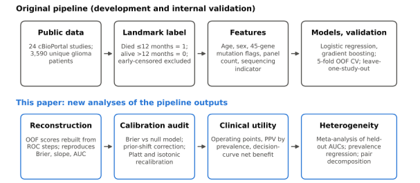
Figure 1: Study Design. Top Row: The Original Pipeline (Development and Internal Validation). Bottom Row: The Secondary Analyses Reported Here, All Computed from The Pipeline's Exported Summary Artefacts.

Data Sources and Cohort Assembly

All data are open access and were obtained from the public cBioPortal REST API, no credentialed or restricted data were used [9,10]. Twenty-four source studies contributed, including MSK-IMPACT cohorts, TCGA glioblastoma and diffuse-glioma cohorts, the GLASS consortium, CPTAC, DKFZ and UCSF series, and several smaller sets [11-13]. Patients were selected by a cancer-type match (gliom | glioblast | astrocytom | oligodendrogli | GBM | DIPG | glioneuron | ependymom) among those carrying an overall-survival endpoint. Individuals appearing in more than one study release were counted once, using an identifier-namespace rule (MSK-IMPACT P#######, TCGA barcodes, TARGET identifiers) [5,6]. The result is 3,590 unique patients.

Institution labels are derived from the same identifier namespace, not from the study. One study can therefore contain patients attributed to different institutions (for example, glioma_ mskcc_2019 contains 531 patients labelled MSK and 138 labelled unattributed), and 1,015 patients carry no attributed institution. Leave-one-study-out validation (Section 2.4) is consequently not leave-one-institution-out validation.

Endpoint

The outcome is a 12-month landmark all-cause mortality label derived from overall-survival status and time: died within 12 months = 1, known to be alive beyond 12 months = 0. Patients censored before 12 months, whose status at the horizon is unknown, were excluded from the binary analysis [20]. The reported prevalence therefore describes patients whose 12-month status is known, and studies with shorter follow-up contribute proportionally fewer survivors.

Features

Clinical features were age at diagnosis in years (available for 94.2%, median-imputed within each training fold) and sex. Genomic features were binary mutation flags for a 45-gene pan¬cancer driver panel, the total number of panel mutations, and a binary indicator of whether the patient had panel sequencing at all. Mutations were taken from each study's mutation profile and aggregated to the patient level as the union across samples and releases. Panel sequencing was available for 2,787 patients (77.6%), for sequenced patients an absent flag is a true wild-type 0. In all there are 49 candidate parameters (age, sex, 45 gene flags, mutation count, sequencing indicator).

What the feature set does not contain matters for interpretation: tumour grade and histology, IDH2 status, 1p/19q co-deletion, copy-number alterations (so EGFR amplification and CDKN2A/B deletion are invisible), TERT promoter status, MGMT methylation, extent of resection and treatment.

Models and the Original Validation Design

Two models were fitted with scikit-learn: L2-regularised logistic regression and histogram-based gradient boosting, both with balanced class weights, so that the two outcome classes contribute equally to the training loss [21]. Numeric features were median-imputed and standardised within each training fold. The primary model was the one with the higher out-of-fold AUC. Internal validation used 5-fold stratified cross-validation with out-of-fold predictions pooled across folds. AUC confidence intervals came from 2,000 bootstrap resamples. The pipeline also reported the area under the precision–recall curve (AUPRC), the Brier score, a 10-bin reliability table, and the calibration slope and intercept from a logistic regression of the outcome on the logit of the predicted probability [23,25]. A clinical-only model (age and sex) served as the ablation baseline. Cross-study robustness was assessed by leave-one-study-out validation: train on all studies but one, test on the held-out study, for the six studies with at least 150 patients and at least 10 patients in each outcome class. Feature importance was measured by permutation importance (loss in AUC). All of this was produced by one reproducible script (evaluation/glioma_ paper.py).

Exported Artefacts Used for the Secondary Analyses

The secondary analyses use only the pipeline's exported files: metrics. Json (reported metrics, ablation, calibration, leave-one-study-out and importance values), table1.json (cohort description), roc_points.csv (1,383 rows of false-positive rate, true-positive rate and score threshold for the primary model's out-of-fold predictions), calibration.csv (ten equal-count bins), leave_one_ source_out.csv, feature_importance.csv and cohort_provenance. csv. No patient-level data, covariates or predictions were available.

Reconstruction of the Out-of-Fold Score Distribution

The ROC table gives, at each distinct score threshold, the cumulative false-positive and true-positive rates. Multiplying successive differences by the totals (770 events, 2,820 non-events) gives the number of events and non-events whose out-of-fold score lies between consecutive thresholds. Each such group was assigned the midpoint of its two bounding thresholds and expanded into pseudo-observations, giving 3,590 (score, outcome) pairs.

The table is thinned, because collinear ROC points are dropped by the standard implementation. Inside a thinned segment individual scores are therefore replaced by the segment midpoint. This leaves the ROC polygon, and so the AUC, exactly unchanged, and perturbs score-dependent quantities (Brier score, calibration slope) only slightly. The reconstruction was validated by comparing the recomputed AUC, average precision, Brier score, calibration slope and intercept, and bootstrap intervals with the values the pipeline reported (Section 3.2). Confidence intervals in this paper that depend on the reconstruction use 2,000 bootstrap resamples of the pseudo-observations.

Calibration Audit

The null model assigns the prevalence π = 770/3,590 to every patient and has Brier score π(1 − π). The Brier skill score is BSS = 1 − BS/BSo, where BSo is the null Brier score, it is negative when a model is worse than the null model [23]. We also compared the mean predicted risk with the prevalence (calibration-in-the-large). With balanced class weights each class contributes equally to the training loss, which is equivalent to training on a population with an outcome prevalence of 0.5. The fitted log-odds are then shifted away from the true log-odds by log((1 − π)/π), and the probabilities are too high whenever π < 0.5 [18,19].

The matching prior-shift correction is \operatorname{logit} p_{\ text{corrected}} = \operatorname{logit} p_{\text{raw}} + \log\ frac{\pi}{1-\pi} It has no parameters fitted from outcomes other than the overall prevalence π. We compared it with Platt scaling (logistic regression of the outcome on the logit of the raw score) and with isotonic regression, each evaluated by 10-fold cross-validation on the pseudo-observations to avoid optimism, the in-sample Platt fit is shown for reference [26]. Metrics were the Brier score, BSS, log-loss, calibration slope and intercept, and the expected calibration error (ECE: the size-weighted mean absolute difference between mean predicted and observed frequency over ten equal-count bins), the maximum calibration error, and the Murphy decomposition of the Brier score into reliability, resolution and uncertainty [24]. Observed frequencies in reliability plots carry Wilson 95% intervals [27].

Operating Characteristics and Decision-Curve Analysis

Operating points were set at 80%, 90% and 95% specificity (quantiles of the non-event scores) and at the Youden optimum. For each we computed sensitivity, specificity, positive and negative predictive value (PPV, NPV) and likelihood ratios, with bootstrap intervals for sensitivity, and expressed the raw score threshold as a calibrated risk through the fitted Platt mapping. Predictive values depend on prevalence. To show how much, we transported each operating point to the mortality of each contributing study using Bayes' rule, PPV = Se·π′ / (Se·π′ + (1 − Sp)(1 − π′)), holding sensitivity and specificity fixed. This is an illustration, not a prediction: sensitivity and specificity themselves vary with case-mix [28].

Decision-curve analysis evaluates the net benefit of acting on patients whose predicted risk is at least a threshold t: \mathrm{NB} (t) = \frac{TP(t)}{N} - \frac{FP(t)}{N}\cdot\frac{t}{1-t}

The treat-all strategy has NB = π − (1 − π)·t/(1 − t), treat-none has NB = 0. The net reduction in unnecessary actions per 100 patients relative to the best default strategy is (NB _oae − max(NB_a 0)) / (t/(1 − t)) × 100. We compared the cross-validated Platt-recalibrated model with the raw scores used as if they were probabilities, with a 95% band from 1,000 bootstrap resamples conditional on the recalibrated predictions.

Heterogeneity and Pair Decomposition

The standard error of each held-out-study AUC was computed from the Hanley–McNeil formula [22]. The six AUCs were pooled by random-effects meta-analysis on the logit scale (DerSimonian–Laird, delta-method variance SE²/[A(1 − A)]²), reporting τ², Cochran's Q, I², a Hartung–Knapp interval and the 95% prediction interval for the AUC in a new study (t distribution, k − 2 degrees of freedom) [29-31]. Sensitivity analyses repeated the pooling on the raw AUC scale and omitting each study in turn, and compared unweighted, event-weighted and pair-weighted means (pairs = events × non-events).

To ask whether discrimination depends on study mortality, we computed Spearman and Kendall rank correlations with exact permutation p values (all 720 permutations of k = 6), and fitted a fixed-weight meta-regression of logit AUC on logit prevalence with residual-variance scaling and t inference on k − 2 = 4 degrees of freedom. With six studies this is an exploratory, ecological analysis.

The pooled AUC is the fraction of concordant case–control pairs among T = 770 × 2,820 = 2,171,400 pairs. A study with e events among n patients contributes e(n − e) within-study pairs, the remaining B = T − W pairs compare patients from different studies. Then \mathrm{AUC}_{\text{pooled}} = \frac{W\,A_ {w} + B\,A_{b}}{W + B} where A_v and A^b are the AUCs of the within-study and between-study pairs. We estimated A_v from the six leave-one-study-out AUCs, weighted by pairs, bounding the contribution of the 18 smaller studies by assuming their within-study AUC to lie between 0.5 and 0.9, and solved for A^bThe step assumes that a leave-one-study-out AUC approximates the within-study AUC of the pooled model, Section 3.6 quantifies the sensitivity to that assumption.

Sample Size, Software and Reporting

Sample-size adequacy for development was checked against the shrinkage criterion of Riley and colleagues, using the Cox–Snell R² of the cross-validated recalibrated predictions, 49 candidate parameters and a target shrinkage of 0.9. This is approximate for gradient boosting, where the parameter count is not defined. Analyses used Python 3 with NumPy, SciPy and scikit-learn, figures used Matplotlib, the random seed was fixed [34]. Reporting follows TRIPOD+AI for prediction-model development with internal validation only (Data, code, reporting and declarations) [21,15].

Results

Cohort and Discrimination

The cohort comprises 3,590 patients from 24 studies, of whom 770 (21.4%) died within 12 months (Table 1). Mean age was 48.3 years (SD 18.5, recorded for 94.2%), 59.6% were male and 77.6% had panel sequencing. The most frequent panel alterations were TP53 (36.5%), IDH1 (29.0%), PTEN (21.7%), EGFR (15.5%) and PIK3CA (10.0%).

Characteristic	Value
Patients (unique)	3,590
Source studies	24
Deaths within 12 months	770 (21.4%)
Age, years, mean ± SD (available for 94.2%)	48.3 ± 18.5
Male sex	59.6%
Panel sequencing available	2,787 (77.6%)
Panel mutations per patient, mean	1.97
TP53 / IDH1 / PTEN / EGFR / PIK3CA mutated	36.5% / 29.0% / 21.7% / 15.5% / 10.0%
RB1 / NOTCH1 / DNMT3A / ARID1A / BRAF / ATM
/ TET2 mutated	6.7% / 6.6% / 6.2% / 4.7% / 4.0% / 3.7% / 3.5%
Labelled subtype (n)	Glioma 3,019, diffuse glioma 406, low-grade glioma/astrocytoma 73, glioneuronal and neuronal tumours 30, glioblastoma 30, high-grade glioma/astrocytoma 21, DIPG 7, GBM 4

                                                                      Table 1. Cohort Characteristics.

The studies differ greatly in size, mortality and sequencing coverage (Figure 2). Among the six largest studies, 12-month mortality ranged from 6.4% (TCGA diffuse glioma) to 44.1% (TCGA glioblastoma), a test of homogeneity across these six studies and the remaining 18 pooled gave χ² = 370.8 on 6 degrees of freedom (p < 10^-75). Across all 24 studies the observed proportion ranged from 0% to 67%, the extremes arising in studies of fewer than 50 patients. Panel sequencing covered from 0% to 100% of patients per study, and 229 of the 803 unsequenced patients (28.5%) belong to TCGA glioblastoma, the study with the highest mortality among the large ones. By institution label, MSK-IMPACT sources contributed 1,620 patients (24.0% mortality), TCGA sources 955 (27.2%), and sources without an attributed institution 1,015 (12.0%).

                                                                       Figure 2: Cohort Composition

(a) Patients per study, split by availability of panel sequencing. (b) 12-month mortality per study with Wilson 95% intervals, the dashed line is the pooled prevalence of 21.4%. The twelve smallest studies (30 patients or fewer each) are pooled in the last row.

The primary gradient-boosting model reached an out-of-fold AUC of 0.774 (95% CI 0.756–0.792), with AUPRC 0.445 and Brier score 0.190 (Table 2). Logistic regression gave 0.770 (0.752–0.787). The clinical-only model of age and sex reached 0.734 (0.715–0.754). The AUPRC of 0.445 is 2.1 times the no-skill level, which equals the prevalence of 0.214.

Model	AUC (95% CI)	AUPRC	Brier score
Logistic regression	0.770 (0.752–0.787)	0.420	0.200
Gradient boosting (primary)	0.774 (0.756–0.792)	0.445	0.190
Clinical only (age, sex)	0.734 (0.715–0.754)	not reported	not reported

                                 Table 2. Out-of-Fold Discrimination (5-Fold Cross-Validation, 2,000-Sample Bootstrap Intervals).

The ROC curve rises steeply at low false-positive rates but flattens at high ones (Figure 3a). Discrimination in the high-specificity region, where a flagged patient would be treated as high-risk, is modest: the McClish standardised partial AUC for false-positive rates up to 0.10 is 0.58, where 0.50 is chance and 1.0 is perfect. Sensitivity is 0.54 at 80% specificity, 0.36 at 90% and 0.21 at 95%. The precision–recall curve (Figure 3b) peaks near 0.6 at very low recall and declines steadily to the prevalence [36,37].

                         Figure 3: Discrimination of the Primary Model (5-Fold Out-of-Fold Predictions).

(a) ROC curve with a 95% bootstrap band and four operating points.

(b) Precision–recall curve with the no-skill line at the prevalence.

Reconstruction Check

The score distribution rebuilt from the ROC steps reproduces every metric the pipeline reported (Table 3). The AUC is identical to four decimals, as it must be, because the ROC polygon is preserved. The Brier score, calibration slope and calibration intercept, which depend on the score values themselves and not only on their ranks, agree to within 0.002. The pipeline's own ten-bin reliability table gives an expected calibration error of 0.187, the same as the reconstruction. Bootstrap interval limits differ by up to 0.0015, which is the order of Monte Carlo variation in 2,000 resamples.

Quantity	Reported by pipeline	Reconstructed
AUC	0.7742	0.7742
AUC, 95% bootstrap CI	0.7562–0.7920	0.7555–0.7905
Average precision (AUPRC)	0.4450	0.4457
Brier score	0.1902	0.1903
Calibration slope	0.7131	0.7141
Calibration intercept	−1.1354	−1.1365
Expected calibration error, 10 bins	0.187 (from reliability table)	0.187
Mean predicted risk	0.396 (mean of bin means)	0.397

            Table 3. Reported Metrics Against the Same Metrics Recomputed from The Reconstructed out-of-FolScores

The agreement on the two calibration parameters is the strongest check, because they would shift if the within-segment scores were materially wrong. We therefore treat the reconstructed distribution as an adequate stand-in for the out-of-fold predictions for the analyses that follow. It is not the predictions themselves. Individual patient identities and covariates are lost, so subgroup analyses (by sex, age or IDH status) and paired tests between models cannot be done from these files (Section 5).

Calibration: The Raw Probabilities Are Worse Than the Null Model

The Raw Predictions Run Far Too High: The mean predicted 12-month mortality is 0.397 against an observed 0.214, so the model predicts almost twice as many deaths as occurred (Figure 4a). Predictions pile up in two regions, near zero and around 0.6, and the highest-risk decile, with a mean prediction of 0.84, has an observed mortality of 0.52 (Figure 5a). Every decile from the fifth upward is over-predicted by 0.16 to 0.32, and the expected calibration error is 0.187. The calibration slope of 0.71 says the predictions are also too spread out, and the intercept of −1.14 says their level is too high.

Figure 4: (a) Raw Out-Of-Fold Predicted Probabilities by Outcome, The Dashed Line Marks the Mean Predicted Risk, Nearly Double the Observed 21.4%. (b) Mappings from Raw to Recalibrated Probability: The Parameter-Free Prior-Shift Correction and The Fitted Platt Mapping. A Raw Prediction of 0.80 Corresponds to A Recalibrated Risk of About 0.46, and 0.50 to about 0.24.

The Brier Score is Worse than that of a Model that Knows Nothing

A model predicting the 21.4% prevalence for every patient has a Brier score of 0.168. The pipeline's reported 0.190 is higher, a Brier skill score of −12.9% (−13.0% on the reconstruction), and the bootstrap 95% interval for the Brier score, 0.183 to 0.198, excludes the null value. The log-loss tells the same story: 0.551 against 0.520 for the null model. The Murphy decomposition shows why. The score carries real information, a resolution term of 0.027, but its reliability error of 0.049 more than cancels it. Discrimination and calibration are separate properties: the AUC of 0.774 and the harmful Brier score belong to the same predictions.

 The Cause is Class Weighting, and it is Correctable Without Fitting Anything

Balanced weights make the training prevalence 0.5, which shifts the log-odds by log(π/(1 − π)) = −1.30 for π = 0.214 [18, 19]. Applying that shift alone moves the mean predicted risk from 0.397 to 0.206 (calibration-in-the-large −0.009), the Brier score from 0.190 to 0.143 (skill +15.4%), the log-loss from 0.551 to 0.443, and the ECE from 0.187 to 0.026 (Table 4, Figure 5b). The only quantity used from the outcomes is the prevalence. The calibration slope is unchanged by any shift, so a residual over-spread remains at the top of the range: the highest decile is predicted at 0.60 and observed at 0.52.

Figure 5: Reliability in Ten Equal-Count Bins (n = 359 each) With Wilson 95% Intervals. (a) Raw Predictions. (b) After the Prior-Shift Correction. (c) After 10-Fold Cross-Validated Platt Scaling.

Cross-validated Platt scaling fixes the remaining over-spread: the calibration slope becomes 0.99, the Brier score 0.142 (skill +15.9%), the ECE 0.018 and the largest decile error 0.035. Isotonic regression gives a similar Brier score (0.142) and ECE (0.017) but a lower slope (0.92) and, because it turns the score into a step function, a lower AUC (0.767 against 0.774). The in-sample Platt fit has Brier score 0.1415, so the optimism of the cross-validated figure is about 0.0002. We therefore recommend Platt scaling, or the prior-shift correction as a transparent default when no recalibration data are available.

Predictions	Brier	Brier skill vs null	Log-lo ss	ECE	Max decile error	Slope	Mean prediction − prevalence	AUC
(prevalence for all)	0.168	0.0%	0.520	n/a	n/a	n/a	0.000	0.500
Raw (class-weighted)	0.190	−13.0%	0.551	0.187	0.321	0.71	+0.182	0.774
Prior-shift only	0.143	+15.4%	0.443	0.026	0.078	0.71	−0.009	0.774
Platt, 10-fold CV	0.142	+15.9%	0.436	0.018	0.035	0.99	0.000	0.774
Isotonic, 10-fold CV	0.142	+15.7%	0.436	0.017	0.044	0.92	0.000	0.7

Table 4. Calibration and Overall Performance of the Raw Predictions, Two Recalibrations and the Null Model.

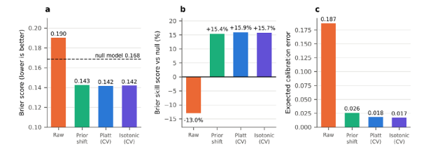
Figure 6: (a) Brier Score, the Dashed Line Is the Null Model. (b) Brier Skill Score Against the Null Model. (c) Expected Calibration Error.

One feature survives recalibration. In the three lowest-risk deciles the observed mortality is 3.9%, 3.1% and 2.2%, which is flat and not monotone with the score, and the lowest decile is under-predicted even after Platt scaling (observed 3.9%, predicted 1.5%, Wilson interval 2.3% to 6.4% for 14 deaths among 359 patients). Among roughly 1,080 patients with the lowest scores the model therefore does not separate patients at risk of early death from those not at risk, a point taken up in the Discussion.

Operating Points, Predictive Values and Decision-Curve Analysis

Operating Points. Table 5 gives the characteristics at four thresholds. At 90% specificity the model flags patients whose recalibrated risk is at least 0.38, it then catches 36% of the deaths (95% CI 32–40%), and about half of the patients it flags (PPV 0.50) die within 12 months. At the Youden optimum the model is a rule-out tool instead: sensitivity is 0.90, but only 34% of flagged patients die. The 43% of patients who fall below the Youden threshold (recalibrated risk 0.17) have a 12-month survival of 95%, a negative likelihood ratio of

Operating point	Raw threshol d	Calibrate d risk threshol d	Sensitivity (95% CI)	Specificit y	PPV	NPV	LR+	LR−
80% specificity	0.628	0.318	0.542 (0.496–0.588)	0.801	0.426	0.865	2.72	0.57
90% specificity	0.709	0.377	0.358 (0.319–0.399)	0.900	0.496	0.837	3.60	0.71
95% specificity	0.783	0.445	0.214 (0.168–0.252)	0.950	0.541	0.816	4.32	0.83
Operating point	Raw threshol d	Calibrate d risk threshol d	Sensitivity (95% CI)	Specificit y	PPV	NPV	LR+	LR−
Youden optimum	0.341	0.167	0.904	0.524	0.342	0.952	1.90	0.18

                        Table 5. Operating Points of the Primary Model (Out-Of-Fold, Calibrated Risk from the Platt Mapping).

Even at 95% specificity a positive prediction is right only 54% of the time, because a likelihood ratio of 4.3 applied to a prior odd of 0.27 gives posterior odds of only 1.2. The model shifts risk, it does not isolate a group that will certainly die.

Predictive Values are not Portable Across Studies:

Predictive values depend on prevalence, and the contributing studies differ more than six fold in 12-month mortality. Holding the 90%-specificity operating point fixed, the PPV would be 0.20 in a study with the mortality of TCGA diffuse glioma (6.4%) and 0.74 in one with the mortality of TCGA glioblastoma (44.1%), while the NPV moves from 0.95 to 0.64 (Table 6, Figure 7). A single quoted PPV or NPV is therefore meaningless without the prevalence it refers to.

Study	12-month mortality	PPV at 80% / 90% / 95% specificity	NPV at 80% / 90% / 95% specificity
TCGA diffuse glioma	6.4%	0.16 / 0.20 / 0.23	0.96 / 0.95 / 0.95
GLASS 2019	6.6%	0.16 / 0.20 / 0.23	0.96 / 0.95 / 0.95
GLASS	8.4%	0.20 / 0.25 / 0.28	0.95 / 0.94 / 0.93
Glioma MSKCC 2019	12.0%	0.27 / 0.33 / 0.37	0.93 / 0.91 / 0.90
MSK-IMPACT 50k	32.3%	0.56 / 0.63 / 0.67	0.79 / 0.75 / 0.72
TCGA glioblastoma	44.1%	0.68 / 0.74 / 0.77	0.69 / 0.64 / 0.

                 Table 6. Predictive Values at Fixed Sensitivity and Specificity, Transported to the Mortality of Each Large Study.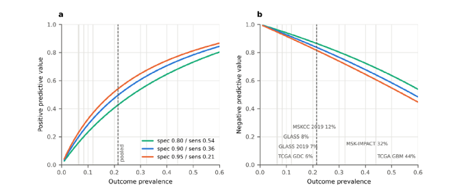

Figure 7: Positive. (a)Negative (b) Predictive Value as a Function of Outcome Prevalence at Three Operating Points of Fixed Sensitivity and Specificity. Vertical Lines Mark the Mortality of the Six Large Studies, The Dashed Line is the Pooled Prevalence. The Assumption of Constant Sensitivity and Specificity Is an Illustration, Not A Prediction.

Decision-Curve Analysis

Net benefit asks whether acting on the model's predictions beats treating everyone or no one, at a given exchange rate between missed deaths and unnecessary actions. With recalibrated risks, the model's net benefit exceeds that of the best default strategy at every threshold from 0.04 to 0.59 on the grid, and the 95% bootstrap band stays above the default from 0.08 to 0.48 (Table 7, Figure 8). At a threshold of 0.20 the model flags 52 of 100 patients and has a net benefit of 0.098 (band 0.083–0.113) against 0.018 for treating everyone: relative to the best default, it avoids 32 unnecessary actions per 100 patients at the same number of deaths covered. At a threshold of 0.30 the gain is 12 per 100, at 0.40 it is 4, and above about 0.48 the band includes zero

Threshold	Flagged per 100	Net benefit, recalibrated (95% band)	Net benefit, raw scores as probabilities	Net benefit, treat all	Unnecessar y actions avoided per 100, recalibrated	Same, raw scores
0.10	64.6	0.152 (0.136–0.166)	0.149	0.127	22.3	19.8
0.20	52.4	0.098 (0.083–0.113)	0.092	0.018	32.0	29.5
0.30	31.5	0.050 (0.036–0.062)	0.029	−0.122	11.6	6.9
0.40	13.3	0.026 (0.015–0.036)	−0.047	−0.309	3.9	−7.1
0.50	4.8	0.006 (−0.001–0.014)	−0.115	−0.571	0.6	−11.5

                                   Table 7. Net Benefit and Net Reduction in Unnecessary Actions at Selected Thresholds.

The cost of skipping recalibration is visible here as well. Used at face value, the raw scores match the recalibrated model at low thresholds (net benefit 0.149 against 0.152 at 0.10), because there most patients are flagged under both. At a threshold of 0.30 the raw scores lose about 40% of the benefit, and from a threshold of 0.35 onward their net benefit falls below zero: acting on them is worse than treating no one, and at 0.40 and 0.50 it causes 7 and 12 net unnecessary actions per 100 patients. This is the decision-level counterpart of the Brier score being worse than the null model.

Figure 8: (a) Decision Curves. The Blue Band is A 95% Bootstrap Interval Conditional on the Cross-Validated Recalibration.

(b) Net Reduction in Unnecessary Actions Per 100 Patients Relative to the Best Default Strategy, with Recalibrated and Raw Scores.

These curves say nothing about which clinical action is appropriate, and the threshold is a clinical judgement that this analysis cannot supply. Illustrative actions might be early palliative-care planning, enrichment of early-phase trials or intensified surveillance. Each implies a different exchange rate and therefore a different threshold.

Cross-Study Heterogeneity

The Headline Range Hides the Precision of Each Estimate: When each of the six largest studies was held out in turn, the AUC ranged from 0.685 to 0.843 (Table 8, Figure 9). That range mixes estimates of very different precision. The three highest values come from studies with 12 to 26 deaths and Hanley–McNeil standard errors of 0.05 to 0.07, so their intervals are up to 0.28 wide and all include the pooled out-of-fold AUC of 0.774. The two largest studies, MSK-IMPACT and TCGA glioblastoma, contribute 518 of the 662 events (78%) and have the lowest AUCs, 0.710 and 0.685, with narrow intervals that exclude 0.774.

Held-out study	Patients	Deaths	12-month mortality	AUC	SE	95% CI
MSK-IMPACT 50k (2026)	896	289	32.3%	0.710	0.019	0.672–0.748
Held-out study	Patients	Deaths	12-month mortality	AUC	SE	95% CI
Glioma MSKCC 2019	669	80	12.0%	0.805	0.030	0.745–0.864
TCGA glioblastoma	519	229	44.1%	0.685	0.024	0.639–0.732
TCGA diffuse glioma (GDC)	406	26	6.4%	0.840	0.049	0.744–0.936
GLASS	309	26	8.4%	0.811	0.052	0.709–0.914
GLASS 2019	182	12	6.6%	0.843	0.072	0.701–0.984

                Table 8. Leave-One-Study-Out Discrimination, with Hanley–McNeil Standard Errors and Intervals.

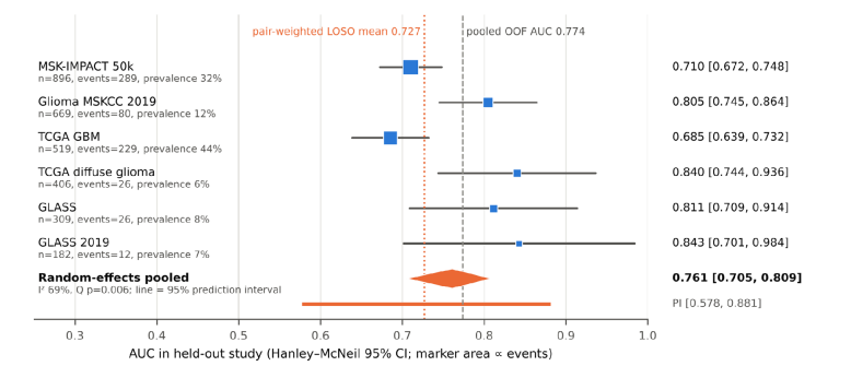
Figure 9: Leave-One-Study-Out AUC Per Held-Out Study (Hanley–McNeil 95% intervals, marker area proportional to the number of events). the orange diamond is the random-effects pooled AUC on the logit scale, the orange line is its 95% prediction interval for a new study. the dashed grey line is the pooled out-of-fold AUC, the dotted orange line is the pair-weighted mean of the six values.

The Held-Out AUCs are Heterogeneous, and the Expected AUC at a New Site is Uncertain: Random-effects pooling on the logit scale gives an AUC of 0.761 (95% CI 0.705–0.809, Hartung–Knapp interval 0.681–0.826). Between-study heterogeneity is substantial: Cochran's Q = 16.2 on 5 degrees of freedom (p = 0.006), I² = 69%, τ² = 0.071 on the logit scale. The 95% prediction interval for the AUC in a new study is 0.578 to 0.881. Pooling on the raw AUC scale gives the same picture (0.768, I² 75%, prediction interval 0.592–0.944). Dropping each study in turn moves the pooled estimate between 0.743 (without Glioma MSKCC 2019) and 0.789 (without TCGA glioblastoma), with I² between 61% and 74%. How the six values are averaged also matters. The unweighted mean is 0.782, pulled up by the three small studies. The event-weighted mean is 0.725 and the pair-weighted mean 0.727, and the two largest studies alone give 0.703. For a randomly chosen pair of one survivor and one non-survivor, the pair-weighted figure is the relevant one.

Discrimination Falls with Study Mortality: Ranking the six studies by 12-month mortality almost perfectly reverses their ranking by AUC (Spearman ρ = −0.94, exact two-sided p = 0.017, the smallest value attainable with six studies, Kendall τ = −0.87, p = 0.017). A meta-regression of logit AUC on logit prevalence has a slope of −0.36 per logit unit (95% CI −0.61 to −0.11, p = 0.016) and leaves no residual heterogeneity (Q = 0.29 on 4 degrees of freedom, p = 0.99, weighted R² 0.98). The fitted curve implies an AUC of about 0.84 at 6.5% mortality, 0.80 at 12%, 0.76 at 21%, 0.72 at 32% and 0.68 at 44% (Figure 10a). The prevalence of 12-month mortality itself varies strongly across these six studies (I² of the log-odds 98%).

Figure 10: (a) Leave-One-Study-Out AUC Against The 12-Month Mortality of The Held-Out Study, With the Meta-Regression Fit And 95% Confidence Band, Marker Area Is Proportional to Events and The Numbers Refer to the studies listed in the panel.

(b) The Pooled Out-Of-Fold AUC Alongside the Implied Between-Study and Within-Study AUCs and the Pair-Weighted AUCs Of the Large Studies (Section 3.6).

This association should be read with three cautions. There are only six points, the analysis is ecological, so it describes studies and not patients, and it was not pre-specified. The AUC is not mathematically tied to prevalence, so mortality here must stand in for something else, most plausibly case-mix and follow-up. A glioblastoma-enriched study contains mostly older patients with IDH-wildtype tumours who are all at high risk, so the model must separate patients within a narrow band of risk. A lower-grade study contains few early deaths, whose age and mutation profile differs markedly from the bulk. Both statements are hypotheses that patient-level covariates would be needed to test.

Pooled Versus Within-Study Discrimination

The pooled out-of-fold AUC of 0.774 is the fraction of concordant case–control pairs among 770 × 2,820 = 2,171,400 pairs. Only 314,051 of these (14.5%) pair patients from the same study, the remaining 1,857,349 (85.5%) pair a patient from one study with a patient from another (Table 9). The six large studies account for almost all within-study pairs (308,231), and the 18 smaller studies for only 5,820.

Pair type	Pairs	Share of all pairs
Within the same study, six large studies	308,231	14.2%
Within the same study, 18 smaller studies	5,820	0.3%
Between studies	1,857,349	85.5%
All pairs	2,171,400	100%

                                                       Table 9. Where the Case–Control Pairs Come From.

If the within-study AUC of the pooled model is approximated by the pair-weighted leave-one-study-out AUC of 0.727, the pooled AUC of 0.774 implies an AUC of 0.782 for between-study pairs (Table 10, Figure 10b). The conclusion does not depend on what is assumed for the 18 small studies, whose pairs are too few to matter: assuming a within-study AUC anywhere from 0.50 to 0.90 for them changes the between-study AUC by less than 0.001.

Comparison	ΔAUC	ρ	SE of Δ	z	p	95% CI for Δ
Genomics added (gradient boosting vs clinical only)	+0.0398	0	0.0134	2.97	0.003	0.014 to 0.066
		0.5	0.0095	4.20	3×10-5	0.021 to 0.058
		0.8	0.0060	6.61	<10-10	0.028 to 0.052
Model choice (gradient boosting vs logistic)	+0.0044	0	0.0128	0.34	0.73	−0.021 to 0.030
		0.5	0.0091	0.49	0.63	−0.013 to 0.022
		0.8	0.0057	0.77	0.44	−0.007 to 0.

  Table 11. Conservative tests of AUC Differences from the Published Bootstrap Intervals, for Assumed Correlation Ρ Between the Paired AUC Estimates.

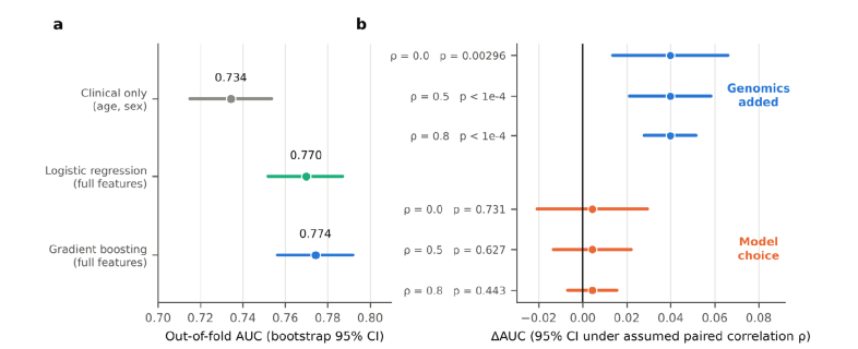
Figure 11: (a) Out-of-Fold AUC With Bootstrap 95% Intervals for The Clinical-Only Model, Logistic Regression and Gradient Boosting. (b) Difference in AUC with 95% Intervals Under Assumed Correlations Of 0, 0.5 And 0.8 Between the Paired Estimates: Adding Genomics (Blue) And Choosing Gradient Boosting Over Logistic Regression (Orange).

Age and IDH1 Carry Most of the Signal: Permutation importance is dominated by age (0.171) and IDH1 mutation (0.121), which together make up 74% of the summed importance of the top 15 features (0.392 in total, Figure 12a). They are followed by TP53 (0.024), the panel mutation count (0.023) and PIK3CA (0.008). The remaining ten features each contribute no more than 0.0062 (median 0.005 for ranks 3–15). No uncertainty was reported for permutation importance, so differences among those small values cannot be separated from noise.

Two features of the importance list deserve attention. First, six of the top 15 features are genes associated with haematological malignancy: GATA2, DNMT3A, ASXL1, KMT2A, TET2 and CBL. Together they carry 0.028, about 56% of the 0.050 carried by the six other genes in the list (TP53, PIK3CA, RB1, CTNNB1, PTEN, NOTCH1). Variants in DNMT3A, TET2 and ASXL1 are the classical markers of age-related clonal haematopoiesis, which is detectable in sequencing of solid tumours and more frequent with age and prior cytotoxic therapy [38–40]. These variants may therefore act as proxies for age or treatment exposure and not for glioma biology, the data here cannot test that. Second, the sequencing indicator is not among the top 15 (its importance is below 0.003), so the model does not appear to lean on whether a patient was sequenced. The mutation count (0.023) may reflect hypermutation or differences in panel size and coverage between studies and could act as a study fingerprint.

The frequent EGFR mutation (15.5%) is also absent from the list, as are ARID1A, BRAF and ATM (Figure 12b). In glioblastoma EGFR is altered mostly by amplification and structural rearrangement, which a mutation-flag panel does not capture, so the absence is a statement about the feature set and not about EGFR [6].

Figure 12: (a) Permutation Importance (Loss in AUC) of the 15 Most Important Features, Coloured By Feature Type. (b) Mutation Frequency of the 12 Most Frequently Mutated Panel Genes, Coloured By Whether the Gene Is Among The 15 Most Important Features.

Discussion

• Principal Findings: Age, sex and a compact mutation panel carry real prognostic information about 12-month mortality in glioma, and most of it comes from age and IDH1. Three further findings qualify that result. The raw probabilities are harmful, with a Brier score worse than the null model, and the cause, class weighting, is cheap to correct. The pooled AUC of 0.774 is an optimistic guide to performance at a new site, because 85% of its case–control pairs cross study boundaries and the leave-one-study-out evidence points to about 0.73, with a plausible range for a single new study of 0.58 to 0.88. And discrimination falls as study mortality rises, so the model is least informative in the glioblastoma-enriched settings where mortality is highest.

• What the Model Does and Does Not Show: That age and IDH1 dominate the importance list is the expected result, and the 0.04 AUC gain from genomics over age and sex is credible under conservative assumptions [3-5]. It is also modest. At 90% specificity the model catches 36% of deaths, and at 95% specificity a positive prediction is correct for 54% of patients. For roughly the lowest-risk 30% of patients the observed mortality is flat at 2–4%, so the score does not discriminate there. The model should be read as a way to shift risk, not as a classifier. We did not compare it with published glioblastoma nomograms, which use curated variables such as performance status, extent of resection and MGMT status and different endpoints, so the comparison would not be like for like. A model of age, sex and mutation flags cannot be expected to match them, and its attraction is that it can be applied wherever a targeted panel exists [7,8].

• Class Weighting and the Cost of Reporting AUC Alone.

The pipeline's summary, an internally validated AUC of about 0.77, was accurate and incomplete. It was silent on a Brier score that is 13% worse than predicting the prevalence for everyone (for the logistic model, 0.200, the loss is 19%). Class weighting is a common reflex for imbalanced outcomes, and it is known to damage calibration while leaving ranking unchanged, here the damage is substantial although the imbalance is only moderate (21% events) [18]. The same predictions that give a respectable AUC would, if used at face value as probabilities, produce net harm at threshold probabilities above 0.35 (Figure 8). The lesson is general. For risk prediction, class weights or resampling should be avoided or undone by recalibration, and calibration, the Brier skill score against the null model and decision-curve net benefit should be reported beside the AUC [17,28]. The prior-shift correction used here is attractive because it needs only the prevalence and so cannot overfit, Platt scaling then removes the residual over-spread.

• Pooled Accuracy and Transportability. Pooling studies raises the number of patients and, with it, the share of between-study comparisons. A random split, as in the pipeline's 5-fold cross-validation, leaves each study represented in training and test sets, so the model can exploit study-level regularities such as age profile, sequencing coverage and baseline risk. The leave-one-study-out analysis is the right correction in principle, and it is more informative when its results are combined by their precision than when only their range is quoted. The range of 0.685 to 0.843 suggests uniform generalisation, the random-effects analysis shows a pooled AUC of 0.761, a prediction interval of 0.578 to 0.881, and a pair-weighted mean of 0.727. The recommended framing is therefore internally and cross-study validated with moderate loss and substantial between-study variation, not simply generalises. Two caveats limit even that. Leave-one-study-out is not leave-one-institution-out: MSK-IMPACT sources comprise 1,620 patients across several studies, and TCGA sources 955, so a held-out MSK or TCGA study leaves a closely related one in the training data. The estimates are therefore probably optimistic with respect to a truly new institution. The fall of AUC with study mortality is the most useful lead for future work, and the least secure result of this paper. It rests on six studies, is ecological, and cannot say whether mortality is a marker of case-mix (glioblastoma against lower-grade disease), of follow-up policy, or of sequencing practice. If it holds, it carries a practical message. The place where a prognostic tool might be most wanted, the glioblastoma-enriched setting where one asks who will survive beyond a year, is where this model is weakest (AUC about 0.68), and the setting where it discriminates best (AUC about 0.84) is one where early deaths are rare and predictive values low (PPV 0.16–0.28 at 80–95% specificity). Stratified analyses by IDH status, grade and age band are the obvious next step and need patient-level data.

• Clinical Utility: Decision-curve analysis shows that the recalibrated model beats both default strategies for thresholds from about 0.08 to 0.48. That window covers actions with a moderate harm–benefit ratio, such as early palliative-care planning or trial enrichment, and excludes actions that would be justified only at very high risk. The analysis assumes that the recalibrated probabilities hold at the new site. Given the heterogeneity above, they would need local recalibration, with at least an updated intercept, before any such use.

• The Feature Set: Six of the 15 most important features are genes associated with haematological malignancy. Variants in such genes are frequent in tumour sequencing of older and previously treated patients through clonal haematopoiesis, and may carry information about age or treatment exposure and not about glioma [38-40]. The panel contains no copy-number, TERT promoter, 1p/19q or CDKN2A/B information, all of which define WHO CNS5 types and grades, and its EGFR flag cannot register amplification [1,6]. Adding molecular class, grade, copy number and, where available, MGMT status and extent of resection is the likeliest route to a clinically useful model. The 0.04 AUC gain from the present panel is, as the original analysis noted, a floor and not a ceiling.

• A Methodological Note: Because the exported ROC table includes thresholds, it contains the entire out-of-fold score distribution up to the thinning of collinear points. This allowed a full calibration and decision-curve audit without patient-level data, and the reproduction of five independently reported quantities, including the two calibration parameters, is a strong validity check. The same fact is a caution for data sharing: a ROC curve with thresholds is not only a summary. For public data it is harmless, for patient-level restricted data, sharing it may reveal more than intended. For the same reason, any pipeline that exports predictions alongside its summaries makes paired tests, subgroup analyses and recalibration possible, and we recommend that practice.

Limitations

• The Secondary Analyses Rest on Exported Summaries.

Individual scores inside thinned ROC segments are replaced by segment midpoints, patient-level covariates and identifiers are absent, and bootstrap intervals are conditional on the reconstruction. Paired tests between models, subgroup analyses (sex, age band, IDH status, specimen type) and subgroup calibration were therefore impossible. Their absence is a gap in the evidence, not evidence of homogeneity.

• There is No External or Prospective Validation: Everything is internal cross-validation plus leave-one-study-out within one assembled public dataset. Because institution labels come from identifier namespaces and a study is not an institution, a held-out MSK or TCGA study leaves related studies from the same institution in training, so the cross-study estimates are probably optimistic for a truly new institution. In TRIPOD terms this is development with internal validation only.

• The Endpoint is Narrow: Twelve-month all-cause mortality is a binary landmark label. Patients censored before 12 months are excluded, which can bias the sample towards longer-followed patients and informatively censored studies, no cause-specific or time-to-event model was fitted, and treatment, which influences survival and may follow from the prediction, is not modelled.

• The Features are Coarse and may be Unevenly Measured. Features are mutation presence only. The assumption that an absent flag in a sequenced patient is a true wild-type holds only if the gene was covered by that study's assay, targeted panels and exome sequencing differ in coverage, and a gene outside a panel would appear as a spurious zero. Panel coverage per study was not examined here. Tumour grade, histology, copy number, 1p/19q, TERT, CDKN2A/B, MGMT, extent of resection and treatment are absent.

• The Cohort Is Heterogeneous in Provenance: The 24 studies include different specimen and cohort types, some identifiers (for example csf_msk_2024 and gbm_mayo_pdx_ sarkaria_2019) suggest specimen types other than primary tumour tissue, which was not examined. Subtype is labelled "Glioma" for 3,019 patients, so case-mix cannot be described in WHO terms. Age was missing for 5.8% and median-imputed.

• The Meta-Analytic Results are Fragile: There are six held-out studies. The Hanley–McNeil variance treats each as an independent sample, Der Simonian–Laird intervals are known to be too narrow for small numbers of studies, which is why a Hartung–Knapp interval and a prediction interval is also given, the prevalence regression is ecological, post hoc and has four residual degrees of freedom.

• The Pair Decomposition is Approximate: It equates the leave-one-study-out AUC with the within-study AUC of the pooled model. Table 10 bounds the error, but the decomposition describes the pooled data and not a causal mechanism.

• Decision Curves Use Recalibration Fitted on the Same Data: Cross-validation limits optimism, but the recalibration was fitted on pooled predictions and would need local updating. The threshold range depends on an unspecified clinical action, and acting on a prediction can change the outcome it predicts.

• The Analyses were Not Pre-Registered: The model development was specified in advance for glioma, the audit analyses were chosen after seeing the reported metrics, and the p values should be read as descriptive.

• Temporal and Subgroup Validity is Untested: Studies span more than a decade of sequencing and treatment practice, and no calibration over time or across sex, age or ancestry groups was possible. These limitations change the strength of the conclusions more than their direction. The calibration finding (Brier score worse than null, repair by prior shift) is checked directly against the pipeline's own reported Brier score and calibration table and that the raw Brier score is worse than the null model uses only reported numbers, and the pipeline's own ten-bin table independently implies a recalibrated Brier of at most 0.1415, in line with the reconstruction. The heterogeneity findings and the decision-curve window are the most dependent on the assumptions above.

Proposed Validation Protocol and Recommendations

The findings point to a specific next study, to be run on the patient-level data behind the pipeline. It has eight steps, in this order.

• Repair Calibration before Anything else. Refit without class weights, or apply the prior-shift correction, then recalibrate on a held-out portion. Report the Brier skill score against the null model, the calibration slope and intercept and the ECE with every AUC [17,18].

• Validate by Institution, Not by Study: Group studies into institutions properly (resolving the 1,015 unattributed patients), then hold out each institution in turn. Report per-institution AUC, calibration slope, calibration-in-the-large, Brier skill and net benefit, and combine them by random-effects meta-analysis with prediction intervals [32,33]. Report within-institution and between-institution AUC separately, and the share of pairs of each kind.

• Stratify by Case-Mix: Report discrimination and calibration by IDH status, age band, grade or WHO type where available, sex, specimen type and sequencing coverage, and test directly whether the fall of AUC with study mortality (Figure 10a) survives adjustment for these variables.

• Extend and Test the Feature Set: Add copy-number features (EGFR amplification, CDKN2A/B deletion, chromosome 7 gain and 10 loss), TERT promoter status, 1p/19q, grade and, where present, MGMT status and extent of resection. Compare with the clinical-only baseline using a paired DeLong or bootstrap test on recalibrated predictions, and make logistic regression the reference model. Test the clonal-haematopoiesis hypothesis by repeating the analysis without the six haematological-type genes and with age-adjusted importance.

• Model Time, Not Just a Landmark: Fit a time-to-event model, report time-dependent AUC and calibration at 12 and 24 months, and handle early censoring by inverse-probability-of-censoring weights instead of exclusion.

• Plan for Precision: With a 21% event rate, a validation cohort needs about 100 events (roughly 470 patients) for an AUC standard error of 0.03, and 150 events (about 700 patients) for 0.024 (Figure S1). Three of the six held-out studies here had 26 events or fewer, which is why their intervals are so wide.

• Choose the Clinical Action and its Threshold Range with Clinicians First, then compute net benefit on locally recalibrated predictions, and state the decision it would change.

• Share Predictions, Not Only Metrics, and Register the Analysis Plan: Export out-of-fold predictions with study, institution and covariates under appropriate controls, pre-register the analyses above, and complete the TRIPOD+AI checklist [15].

For any similar model built on pooled public cohorts, five items should accompany the headline AUC: The Brier skill score against the null model, the calibration slope and intercept, per-study AUC with intervals and a prediction interval, the share of case–control pairs that lie within a single study, and the sensitivity and specificity transported to the prevalence of the intended setting.

Conclusions

Age, sex and a compact mutation panel discriminate 12-month mortality in 3,590 patients with glioma from 24 public cohorts with an out-of-fold AUC of 0.774 (95% CI 0.756–0.792), 0.04 above age and sex alone, and almost all of the signal comes from age and IDH1. Four findings qualify that result.

• The raw probabilities are unusable. Their Brier score of 0.190 is worse than the 0.168 of a model predicting the prevalence for everyone, because class weighting inflated every prediction. A prior-shift correction with no fitted parameters brings the Brier score to 0.143, and cross-validated Platt scaling to 0.142.

• The pooled AUC overstates what a new site should expect. 85.5% of its case–control pairs cross study boundaries. Held-out-study AUCs pool to 0.761 (95% CI 0.705–0.809) with a prediction interval of 0.578–0.881, and their pair-weighted mean is 0.727.

• Discrimination falls with study mortality (AUC about 0.84 at 6.5% mortality and 0.68 at 44%), an exploratory finding that needs patient-level data to test.

• After recalibration the model has net benefit above the best default strategy for threshold probabilities from about 0.08 to 0.48, but predictive values depend heavily on prevalence and the model separates risk only modestly.

• The model is not ready for clinical use. Validation by institution, richer molecular features and local recalibration are the necessary next steps (Section 6), and any report of such models should state calibration, per-study heterogeneity and the share of within-study comparisons alongside the AUC.

Data, Code, Reporting and Declarations

Data Availability: All source cohorts are public on cBioPortal, the 24 study identifiers, with per-study counts, are listed in cohort_ provenance.csv and summarised in Figure 2 and Supplementary Table S1. The exported artefacts analysed here (metrics.json, table1.json, roc_points.csv, calibration.csv, leave_one_source_out. csv, feature_importance.csv, cohort_provenance.csv) are available from the authors.

Code Availability: The model pipeline comprises data/download_ pancancer.py, data/download_genomics.py, data/clean_patients. py, data/deduplicate.py, data/build_dev_cohort.py and evaluation/ glioma_paper.py. The scripts for the secondary analyses and figures in this paper (score reconstruction, calibration audit, decision curves, meta-analysis, pair decomposition) are supplied with the manuscript as analysis.py and figures.py, with all numerical results

Reporting Standard: The study follows TRIPOD+AI for prediction-model development with internal validation. It is development with internal and cross-study validation only (TRIPOD type 1b), there is no external validation [15].

Supplementary Material

S1. Per-Study Provenance

Counts per source dataset in the analysed cohort (n = 3,590, 770 deaths within 12 months). Coverage is the share of patients with genomic data.

Study	n	Deaths	Mortality	With genomics	Coverage
msk_impact_50k_2026	896	289	32.3%	734	82%
glioma_mskcc_2019	669	80	12.0%	605	90%
gbm_tcga	519	229	44.1%	290	56%
difg_tcga_gdc	406	26	6.4%	382	94%
difg_glass	309	26	8.4%	253	82%
difg_glass_2019	182	12	6.6%	164	90%
brain_cptac_2020	109	7	6.4%	44	40%
csf_msk_2024	105	25	23.8%	66	63%
gbm_mayo_pdx_sarkaria_2019	102	30	29.4%	70	69%
difg_msk_2023	60	1	1.7%	60	100%
Study	n	Deaths	Mortality	With genomics	Coverage
pancan_hcmi_2025	55	14	25.5%	46	84%
past_dkfz_heidelberg_2013	47	0	0.0%	2	4%
gbm_columbia_2019	30	1	3.3%	12	40%
gbm_iatlas_prins_2019	28	16	57.1%	0	0%
lgg_ucsf_2014	22	0	0.0%	22	100%
msk_impact_2017	13	3	23.1%	7	54%
mycf_msk_2026	11	5	45.5%	9	82%
odg_msk_2017	11	3	27.3%	9	82%
pog570_bcgsc_2020	7	1	14.3%	5	71%
mixed_impact_subset_2022	3	2	66.7%	3	100%
astr_ut_2026	2	0	0.0%	2	100%
gbm_tcga_pub2013	2	0	0.0%	0	0%
lgg_tcga	1	0	0.0%	1	100%
pancan_mimsi_msk_2024	1	0	0.0%	1	100%

By attributed institution: MSK-IMPACT 1,620 patients, 388 deaths, 84.1% with genomics, TCGA 955, 260, 73.2%, unattributed 1,015, 122, 71.5%. Institution is assigned per patient in the provenance export, so a study (for example glioma_mskcc_2019 or difg glass) can appear under more than one institution.

S2. Leave-One-Study-Out Sensitivity of the Pooled Estimate

Random-effects pooling on the logit AUC scale, dropping each of the six held-out studies in turn. The full-data pooled AUC is 0.761 (95% CI 0.705–0.809, Hartung–Knapp 0.681–0.826), with a prediction interval of 0.578–0.881.

Dropped study	Pooled AUC	I²	95% prediction interval
msk_impact_50k_2026	0.787	74%	0.462–0.941
glioma_mskcc_2019	0.743	61%	0.553–0.871
gbm_tcga	0.788	66%	0.529–0.925
difg_tcga_gdc	0.748	68%	0.549–0.879
difg_glass	0.754	72%	0.537–0.890
difg_glass_2019	0.755	72%	0.541–0.889

No single study moves the pooled estimate outside 0.743–0.788, and heterogeneity stays between 61% and 74%. The two large-cohort exclusions (MSK-IMPACT, TCGA glioblastoma) raise the pooled value, excluding the MSKCC 2019 cohort lowers it.

S3. Full Ten-Bin Calibration Table of the Raw Model

Supplied by the pipeline (equal-count bins of 359 patients). Observed frequency is below the predicted probability in nine of ten bins, by 0.30–0.32 in the top four. The binned expected calibration error is 0.187, and the Brier score implied if each bin were recalibrated to its observed rate is at most 0.1415.

Bin	Mean predicted	Observed	n	Gap
1	0.014	0.039	359	−0.025
2	0.047	0.031	359	+0.016
3	0.082	0.022	359	+0.060
4	0.183	0.070	359	+0.113
5	0.369	0.212	359	+0.157
6	0.497	0.248	359	+0.249
7	0.576	0.273	359	+0.303
8	0.639	0.320	359	+0.319
9	0.718	0.412	359	+0.306
10	0.838	0.518	359	+0.320

S4. Derivations

• Prior-Shift Correction. Balanced class weights make the model learn the posterior under an effective prevalence of 0.5. For true prevalence π, the corrected probability is logit(p′) = logit(p) + log(π/(1−π)). With π = 0.2145 the offset is −1.298 (reference 19).

• Hanley–McNeil Standard Error. With Q1 = A/(2−A), Q2 = 2A²/(1+A), SE² = [A(1−A) + (n1−1)(Q1−A²) + (n0−1)(Q2− A²)] / (n1 n0), where n1 and n0 are the numbers of events and non-events (reference 22).

• Murphy Decomposition. Brier = reliability − resolution + uncertainty, with uncertainty π(1−π) = 0.1685 (reference 24). A model whose Brier exceeds this value is worse than issuing the base rate to everyone.

• Pair Decomposition. The pooled AUC counts every event–non-event pair, T = 2,171,400 in total. Pairs from the same study (314,051, 14.5%) have within-study AUC 0.727. Pairs from different studies (1,857,349, 85.5%) have AUC 0.782. The pooled figure is therefore a weighted mixture dominated by between-study comparisons, which are partly easy because study mortality differs.

S5. Sample-Size Check for Model Development (Riley Criteria)

Using 49 candidate parameters and prevalence 0.2145, the Cox–Snell R² from the fitted logistic model is 0.154 (Nagelkerke 0.238, maximum attainable 0.646). Events per predictor parameter are 15.7. The minimum sample size for a shrinkage factor of 0.9 is 2,609, against 3,590 patients available (reference 34).

S6. Precision of AUC by Number of Events

Hanley–McNeil standard error for an AUC of about 0.77 at the stated event counts.

Events	SE of AUC
10	0.094
12	0.085
26	0.058
50	0.042
80	0.033
150	0.024
289	0.017
770	0.011

Figure S1 Plots this Relationship against the Six Held-Out Studies.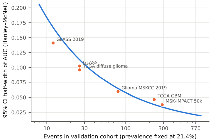

                                                 Figure S1: Precision of Study-Level AUC as a Function f Event Count.

S7. Reconstruction of the Out-of-Fold Score Distribution

Patient-level out-of-fold scores were not available. They were reconstructed from the exported ROC table: each step between consecutive points gives the number of events and non-events falling in that score segment, and segment midpoints stand in for the scores. The reconstruction reproduces the reported metrics closely (reported → reconstructed): AUC 0.7742 → 0.7742, average precision 0.445 → 0.446, Brier 0.1902 → 0.1903, calibration intercept −1.135 → −1.136, calibration slope 0.7131 → 0.7141. Results that depend on the distribution within a segment (ECE, decision curves) inherit a small discretisation error, which is why the Brier-worse-than-null finding is also checked against the pipeline's own ten-bin table (S3).

References

- Louis, D. N., Perry, A., Wesseling, P., Brat, D. J., Cree, I. A., Figarella-Branger, D., ... & Ellison, D. W. (2021). The 2021 WHO classification of tumors of the central nervous system: a summary. Neuro-oncology, 23(8), 1231-1251.
- Stupp, R., Mason, W. P., Van Den Bent, M. J., Weller, M.,Fisher, B., Taphoorn, M. J., ... & Mirimanoff, R. O. (2005). Radiotherapy plus concomitant and adjuvant temozolomide for glioblastoma. New England journal of medicine, 352(10), 987-996.
- Yan, H., Parsons, D. W., Jin, G., McLendon, R., Rasheed,B. A., Yuan, W., ... & Bigner, D. D. (2009). IDH1 and IDH2mutations in gliomas. New England journal of medicine, 360(8), 765-773.
- Eckel-Passow, J. E., Lachance, D. H., Molinaro, A. M., Walsh,K. M., Decker, P. A., Sicotte, H., ... & Jenkins, R. B. (2015). Glioma groups based on 1p/19q, IDH, and TERT promoter mutations in tumors. New England Journal of Medicine, 372(26), 2499-2508.
- Cancer Genome Atlas Research Network. (2015). Comprehensive, integrative genomic analysis of diffuse lower-grade gliomas. New England Journal of Medicine, 372(26), 2481-2498.
- Brennan, C. W., Verhaak, R. G., McKenna, A., Campos, B., Noushmehr, H., Salama, S. R., ... & Davidsen, T. (2013). The somatic genomic landscape of glioblastoma. cell, 155(2), 462-477.
- Gorlia, T., Van Den Bent, M. J., Hegi, M. E., Mirimanoff,R. O., Weller, M., Cairncross, J. G., ... & Stupp, R. (2008). Nomograms for predicting survival of patients with newly diagnosed glioblastoma: prognostic factor analysis of EORTC and NCIC trial 26981-22981/CE. 3. The lancet oncology, 9(1), 29-38.
- Gittleman, H., Lim, D., Kattan, M. W., Chakravarti, A., Gilbert,M. R., Lassman, A. B., ... & Barnholtz-Sloan, J. S. (2017). An independently validated nomogram for individualized estimation of survival among patients with newly diagnosed glioblastoma: NRG Oncology RTOG 0525 and 0825. Neuro-oncology, 19(5), 669-677.
- Cerami, E., Gao, J., Dogrusoz, U., Gross, B. E., Sumer,S. O., Aksoy, B. A., ... & Schultz, N. (2012). The cBio cancer genomics portal: an open platform for exploring multidimensional cancer genomics data. Cancer discovery, 2(5), 401-404.
- Gao, J., Aksoy, B. A., Dogrusoz, U., Dresdner, G., Gross, B., Sumer, S. O., ... & Schultz, N. (2013). Integrative analysis of complex cancer genomics and clinical profiles using the cBioPortal. Science signaling, 6(269), pl1-pl1.
- Cheng, D. T., Mitchell, T. N., Zehir, A., Shah, R. H., Benayed,R., Syed, A., ... & Berger, M. F. (2015). Memorial Sloan Kettering-Integrated Mutation Profiling of Actionable Cancer Targets (MSK-IMPACT): a hybridization capture-based next-generation sequencing clinical assay for solid tumor molecular oncology. The Journal of molecular diagnostics, 17(3), 251-264.
- Zehir, A., Benayed, R., Shah, R. H., Syed, A., Middha, S., Kim, H. R., ... & Berger, M. F. (2017). Mutational landscape of metastatic cancer revealed from prospective clinical sequencing of 10,000 patients. Nature medicine, 23(6), 703-713.
- Kim, Hoon, Roel GW Verhaak, and GLASS Consortium. "Glioma through the looking GLASS: molecular evolution of diffuse gliomas and the Glioma Longitudinal Analysis Consortium." (2018): 873.
- Collins, G. S., Reitsma, J. B., Altman, D. G., & Moons, K.G. (2015). Transparent reporting of a multivariable prediction model for individual prognosis or diagnosis (TRIPOD): the TRIPOD statement. Journal of British Surgery, 102(3), 148-158.
- Collins, G. S., Moons, K. G., Dhiman, P., Riley, R. D., Beam,A. L., Van Calster, B., ... & Logullo, P. (2024). TRIPOD+ AI statement: updated guidance for reporting clinical prediction models that use regression or machine learning methods. bmj, 385.
- Steyerberg, E. W., & Harrell Jr, F. E. (2015). Prediction models need appropriate internal, internal-external, and external validation. Journal of clinical epidemiology, 69, 245.
- Calster, B. (2019). Calibration: the Achilles heel of predictive analytics. BMC Med, 17(1), 1.
- Van den Goorbergh, R., Van Smeden, M., Timmerman, D., & Van Calster, B. (2022). The harm of class imbalance corrections for risk prediction models: illustration and simulation using logistic regression. Journal of the American Medical Informatics Association, 29(9), 1525-1534.
- Saerens, M., Latinne, P., & Decaestecker, C. (2002). Adjusting the outputs of a classifier to new a priori probabilities: a simple procedure. Neural computation, 14(1), 21-41.
- Anderson, J. R., Cain, K. C., & Gelber, R. D. (1983). Analysis of survival by tumor response. Journal of clinical oncology, 1(11), 710-719.
- Pedregosa, F., Varoquaux, G., Gramfort, A., Michel, V., Thirion, B., Grisel, O., ... & Duchesnay, É. (2011). Scikit-learn: Machine learning in Python. the Journal of machine Learning research, 12, 2825-2830.
- Hanley, J. A., & McNeil, B. J. (1982). The meaning and use of the area under a receiver operating characteristic (ROC) curve. Radiology, 143(1), 29-36.
- Glenn, W. B. (1950). Verification of forecasts expressed in terms of probability. Monthly weather review, 78(1), 1-3
- Murphy, A. H. (1973). A new vector partition of the probability score. Journal of Applied Meteorology and Climatology, 12(4), 595-600.
- Cox, D. R. (1958). Two further applications of a model for binary regression. Biometrika, 45(3/4), 562-565.
- Platt, J. (1999). Probabilistic outputs for support vector machines and comparisons to regularized likelihood methods. Advances in large margin classifiers, 10(3), 61-74.
- Wilson, E. B. (1927). Probable inference, the law of succession, and statistical inference. Journal of the American Statistical Association, 22(158), 209-212.
- Vickers, A. J., & Elkin, E. B. (2006). Decision curve analysis: a novel method for evaluating prediction models. Medical Decision Making, 26(6), 565-574.
- DerSimonian, R., & Laird, N. (1986). Meta-analysis in clinical trials. Controlled clinical trials, 7(3), 177-188.
- Hartung, J., & Knapp, G. (2001). A refined method for the meta-analysis of controlled clinical trials with binary outcome. Statistics in medicine, 20(24), 3875-3889.
- IntHout, J., Ioannidis, J. P., Rovers, M. M., & Goeman, J. J. (2016). Plea for routinely presenting prediction intervals in meta-analysis. BMJ open, 6(7), e010247.
- Debray, T. P., Vergouwe, Y., Koffijberg, H., Nieboer, D., Steyerberg, E. W., & Moons, K. G. (2015). A new framework to enhance the interpretation of external validation studies of clinical prediction models. Journal of clinical epidemiology,68(3), 279-289.
- Riley, R. D., Ensor, J., Snell, K. I., Debray, T. P., Altman, D. G., Moons, K. G., & Collins, G. S. (2016). External validation of clinical prediction models using big datasets from e-health records or IPD meta-analysis: opportunities and challenges. bmj, 353.
- Riley, R. D., Ensor, J., Snell, K. I., Harrell, F. E., Martin, G. P., Reitsma, J. B., ... & Van Smeden, M. (2020). Calculating the sample size required for developing a clinical prediction model. Bmj, 368.
- Ransohoff, D. F., & Feinstein, A. R. (1978). Problems of spectrum and bias in evaluating the efficacy of diagnostic tests. New England Journal of Medicine, 299(17), 926-930.
- Saito, T., & Rehmsmeier, M. (2015). The precision-recall plot is more informative than the ROC plot when evaluating binary classifiers on imbalanced datasets. PloS one, 10(3), e0118432.
- McClish, D. K. (1989). Analyzing a portion of the ROC curve Medical decision making, 9(3), 190-195.
- Jaiswal, S., Fontanillas, P., Flannick, J., Manning,A., Grauman,P. V., Mar, B. G., ... & Ebert, B. L. (2014). Age-related clonal hematopoiesis associated with adverse outcomes. New England Journal of Medicine, 371(26), 2488-2498.
- Genovese, G., Kähler, A. K., Handsaker, R. E., Lindberg, J., Rose, S. A., Bakhoum, S. F., ... & McCarroll, S. A. (2014). Clonal hematopoiesis and blood-cancer risk inferred from blood DNA sequence. New England Journal of Medicine, 371(26), 2477-2487.
- Coombs, C. C., Zehir, A., Devlin, S. M., Kishtagari, A., Syed, A., Jonsson, P., ... & Berger, M. F. (2017). Therapy-related clonal hematopoiesis in patients with non-hematologic cancers is common and associated with adverse clinical outcomes. Cell stem cell, 21(3), 374-382.