Design of Intelligent Channelizer for Extracting Signals of Arbitrary Centre Frequency and Bandwidth

Introduction

The traditional approach to wideband signal channelization has been to use a bank of digital down conversion (DDC) units, with each channel being produced individually via a DDC unit which digitally down-converts the signal to base-band, constrains the bandwidth with a digital filter, and then reduces the sampling rate by an amount commensurate with the reduction in bandwidth [1]. This approach is costly, however, in that multiple channels are produced via replication of the DDC unit, so that there is no commonality of processing and therefore no possibility of computational savings being made. This is particularly relevant when the number of channels is large, as each DDC unit typically requires one/two finite impulse response (FIR) low pass filters for real-valued/complex-valued data and one stored period of a complex sinusoid sampled at the input sampling frequency [2,3].

With such a situation a polyphase decomposition may be beneficially used to enable the bank of DDC units, as illustrated in Fig. 1a for the case of a single channel, to be simply transformed into an alternative filter bank structure, namely the polyphase discrete Fourier transform (DFT) or PDFT of Fig. 1b, whereby large numbers of channels may be simultaneously produced at computationally acceptable levels. The major disadvantage of the approach is that the spacing between the fixed-bandwidth channels is uniform so that even relatively narrow bandwidth signals may potentially be spread across more than one channel. This makes the subsequent tasks of signal extraction and demodulation extremely difficult to achieve [1,4,5].

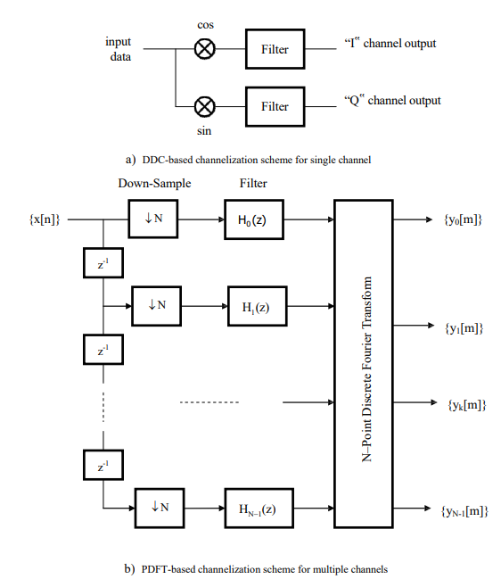
                                  Figure 1: conventional solutions to channelization problem

Thus, there are clear advantages and disadvantages with both approaches in that: a) with the DDC approach, optimal performance and flexibility is obtained but at the expense of a heavy computational load that increases linearly with the number of signals of interest; whereas b) with the PDFT approach, a sub-optimal and less flexible performance is obtained but at a greatly reduced computational cost through the exploitation of a suitably defined fast Fourier transform (FFT) module. A solution that could exploit the merits of both approaches would therefore be very attractive, offering the promise of a hardware implementation with a low size, weight and power (SWAP) requirement.

The research presented in this paper looks at how to address this problem, with Section 2 outlining how the two approaches might be suitably combined and Section 3 discussing how to incorporate into the design a high-resolution FFT with ×4 update rate which might be subsequently used for directing the application of the low-rate DDC units to the relevant PDFT channel outputs. Section 4 discusses how pipelining of the various interconnecting components of the channelization scheme might be achieved, in a synchronised fashion, with the associated complexity requirements being addressed in Section 5 and a summary and conclusions in Section 6. An Appendix is also provided which discusses, in some depth, how a long FFT – for the provision of high-resolution FFT outputs – might be constructed from the piecing together of shorter FFTs.

Optimal Combination of Standard Channelization Techniques

To see how the two standard approaches to wideband signal channelization might be optimally combined a modular design is considered which comprises, essentially, four distinct sub- systems: a) a PDFT module; b) a high-resolution FFT module yielding ×4 update rate; c) a DDC module comprising a bank of DDC units; and d) a signal parameter estimation (SPE)

module which identifies those PDFT channels that contain the signals of interest, in their entirety, together with estimates of the relevant signal parameters – namely, the centre frequencies and bandwidths. Thus, the bank of DDC units, when provided with suitable guidance by the SPE module, operates directly upon the outputs of the PDFT module.

Suppose firstly that the maximum signal bandwidth of interest is denoted by ‘WS’ and that for the operation of the PDFT module the channel bandwidth, ‘WC’, is set to twice this value, so that

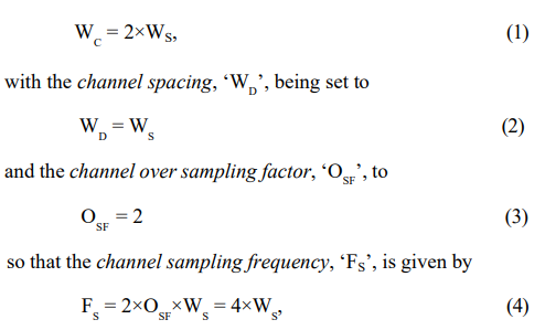
and for every signal of interest there will be at least one channel within which the signal is completely contained. This is clearly evident from examination of Fig. 2a, since as soon as the signal spectrum is shifted past the boundary of one channel, so it moves completely into its overlapping neighbour – the prototype channel filtering requirement is as defined in Fig. 2b.

Figure 2: description of channel bandwidth, spacing and filtering requirements

Thus, if some means is available for determining the frequency locations of those channels that completely contain the signals of interest, then a DDC unit – and possibly a sampling rate converter (SRC) – could be assigned to each such channel to enable the signal to be optimally extracted once the centre frequency and bandwidth of the signal have been estimated via some suitable means. This ability to capture entire signals via individual channels through the appropriate setting of the PDFT parameters is a key feature of the proposed design as it facilitates the intelligent use of the DDC module.

Note that this idea may be extended so that if, for example, there were two distinct signal bandwidths of interest, where one bandwidth is considerably smaller than the other, then the two bandwidths could be catered for by the cascading together of two PDFT systems. With the first system, the defining parameters could be chosen to ensure that each wide bandwidth signal is completely contained by at least one of the resulting wide PDFT channels. With the second system – which operates upon the channelized outputs of the first system – the defining parameters could be similarly chosen to ensure that each narrow bandwidth signal is completely contained by at least one of the resulting narrow PDFT channels.

Another key feature of the proposed design, as described in Fig. 3, is that if a complex-data FFT module is used for the processing of the polyphase filtered data, then it may also be used for the processing of the windowed input data – given that both types of data are assumed to be real-valued – which may subsequently be used by the SPE module. The two data sets may be processed simultaneously through the suitable packing/unpacking of the FFT input/output complex-valued data array, with the PDFT path being referred to in Fig. 3 as ‘Path A’ and the windowed FFT path as ‘Path B’. The ‘Path B’ data, after unpacking, is thus fed to the SPE module which typically carries out averaging, thresholding and interpolation of the squared amplitudes of the spectrum to determine the addresses of those channels that contain the signals of interest [6]. For those particular channels, the unpacked ‘Path A’ data is then passed to the SPE module and a parameter estimation routine executed which involves the channelized data being spectrum analysed to yield estimates of the centre frequency and bandwidth of those signals residing within the channels. This enables the DDC units to be used for optimally extracting the signals of interest from the targeted channels and SRC units to be used, if required, to adjust the output sampling rate from the DDC units to satisfy any future processing requirements.

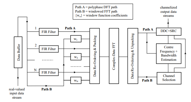
Figure 3: hybrid channelization scheme exploiting low-resolution FFT module

Note that when the oversampling is achieved via overlapping of the input data segments , as is proposed, the application of the ×4 oversampling factor requires that the input data segments be overlapped by a factor of 75% so that, from Fig. 3, only N/4 new samples are to be input to the PDFT input buffer between each update of the N branch polyphase filter. The undesirable phase effects produced by the oversampling – at least when achieved by this particular means – is straightforwardly accounted for by the data reordering stage that immediately follows the polyphase filtering [1].

Guidance of DDC Units via High-Resolution FFT

An alternative approach to the channelization scheme of Fig. 3 involves using the low-resolution windowed FFTs, as produced for use by the SPE module, to instead construct a high-resolution FFT, where the length of the longer FFT is taken to be a multiple of the length of the shorter FFT such that the multiplying factor and the length of the shorter FFT are relatively prime – this type of factorization is referred to in the technical literature as the Prime Factor Algorithm and its derivation discussed in some detail in the Appendix [7]. The length of the FFT is chosen to facilitate the resolution of those signals possessing the minimum signal bandwidth of interest (and thus of all signals of interest). Referring to the scheme displayed in Fig. 4, the FFT processing may be partitioned into two distinct stages: a row- DFT stage,which comprises ‘M’ FFTs each of length ‘N’; and a column- DFT stage, which comprises ‘N’ FFTs each of length ‘M’. The lengths ‘M’ and ‘N’ are assumed, for our purposes, to be such that

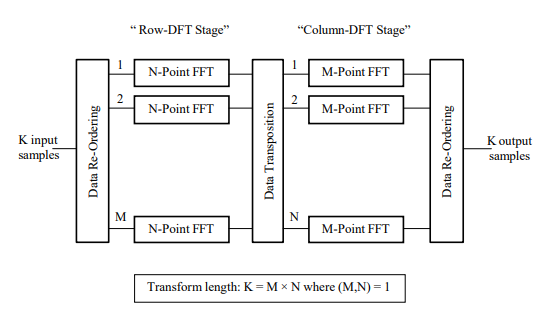
 Figure 4: composite length FFT with relatively prime length factors

    N >> M,                                                                           (5)

so that the M-point FFTs may be referred to as the ‘short’ FFTs and the N-point FFTs as the ‘long’ FFTs. The parameter ‘M’ is thus responsible for determining the increased resolving capability when compared to the original N-point low-resolution FFT scheme.

The resulting channelization scheme is as shown in Fig. 5, whereby two real-valued FFT data sets are still processed simultaneously in the same way as before, but with segments of data now being fed into a suitably sized buffer until there are sufficient samples available for windowing and feeding to the complex-data FFT routine. Once the row-DFT output data sets have been produced by the FFT, they may be fed as input to the column-DFT stage which produces the high-resolution FFT outputs from which, after averaging and thresholding of the squared amplitudes, the signal centre frequency and bandwidth estimates may then be directly obtained. Interpolation could also be again used to enhance the accuracy of the centre frequency estimate yielded by the high resolution FFT.

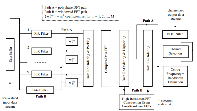
Figure 5: hybrid channelization scheme exploiting high-resolution FFT module

The short M-point FFTs required for the construction of the high-resolution FFT may be carried out in optimal fashion via one of Winograd’s short-DFT algorithms (which are, in turn, based upon the use of optimal fast circular convolution algorithms), with additional savings being potentially obtained by computing only those outputs that correspond to the non- negative frequency components of the required composite length transform [8]. The structure of the optimal short-DFT algorithms – which may each be expressed in the form of a set of pre-weave additions, followed by a set of nested point-wise multiplications, followed by a set of post-weave additions – lends itself naturally to a pipelined implementation.

Thus, the computational complexity of either version of the channelization scheme is kept to a minimum by using the PDFT module to produce a set of relatively wide overlapping channels that cover the entire frequency spectrum. The DDC module, comprising the bank of DDC units, is then applied to the outputs of a subset of the overlapping channels – namely those channels containing the signals of interest – so that the DDC units are applied only at the channel sampling frequency rather than the system sampling frequency.

The high-resolution FFT technique described above – namely, the Prime Factor Algorithm – requires the lengths of the two FFT factors, ‘M’ and ‘N’, to be relatively prime. This simplifies the processing requirements in that the outputs from the row- DFT stage may be fed directly into the column-DFT stage without further modification. An alternative approach may be adopted, however, whereby there is no restriction on the relative lengths of the two FFT factors. The attraction of this approach – referred to as the Common Factor Algorithm (CFA) and whose derivation, like that of the PFA, is discussed in some detail in the Appendix – is that the length of the small M point FFTs may be arbitrarily chosen [9]. The drawback is that if the lengths of the two factors are not relatively prime, then the outputs from the row-DFT stage must first be modified via the application of appropriate pre-computed twiddle factors (accessed from a suitably defined look-up table (LUT)) before being fed to the column DFT stage [2,3].

Pipelined Operation of Hybrid Channelization Scheme

To facilitate the channelization for potentially large numbers of channels, it is assumed that the proposed scheme is to be implemented in a highly-parallel fashion that makes efficient use of pipelining and single-instruction multiple-data (SIMD) multi processing techniques [10]. The target hardware is assumed, for purposes of illustration, to be a field programmable gate array (FPGA) device such that each input sample may be read into its buffer at the rate of one sample per clock cycle [11]. Then every N/4 clock cycles – referred to hereafter as the update time – the input data buffer to the PDFT module is updated with N/4 new samples and the operation of the polyphase filtering – and all subsequent processing – repeated.

Thus, this results in a timing constraint being imposed upon the operation of the proposed channelization scheme in that the time complexity of each sub-system must be such that the outputs can be updated within just N/4 (or some multiple of for the case of the high resolution FFT) clock cycles. This means that each of the sub-systems must be broken down into components which, when suitably pipelined and synchronised, enable this to be achieved.

Double Buffers and Processing Elements

The technique of double buffering will need to be utilized in several places to ensure that pipelined operation of the channelization scheme is achieved. The basic idea is that whilst one buffer is being updated with new data, the data from the other is being processed by the appropriate processing elements (PEs). When the buffer is completely refreshed each time with new data this is quite a straightforward task. When overlapping of the data is involved, however, a more complex scheme is required. To achieve this, new data and data from the buffer being processed are fed simultaneously into the buffer being updated and the operation of the two buffers alternated with the availability of each new set of data – see Fig. 6 for the case of the complex-data FFT.

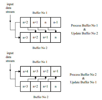
Figure 6: operation of data buffers for input to complex-data FFT

For such operation to be achieved, however, each buffer must be partitioned into the form of a memory bank – there will have to be at least four memories per bank for consistency with the 75% overlapping requirement – with each memory being typically made up from fast, dual-port random access memory (RAM) [11]. In this way, multiple samples may be read/written from/to the memory bank every clock cycle, with one read/write pair or two reads/writes from/to each memory, so that the data may be fed into the appropriate PEs at the required rate for processing to be maintained.

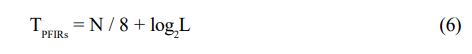
A description of how the pipelining might be achieved is given in Figs. 7 and 8, with two levels of granularity being described for the PEs via the introduction of both course-grain processing elements (CPEs), as shown in Fig. 7, and fine-grain processing elements (FPEs), as shown in Fig. 8. An adequate timing margin will be sought, in each case, to allow for potential delays arising from the pipelined operation of the various interconnecting components.

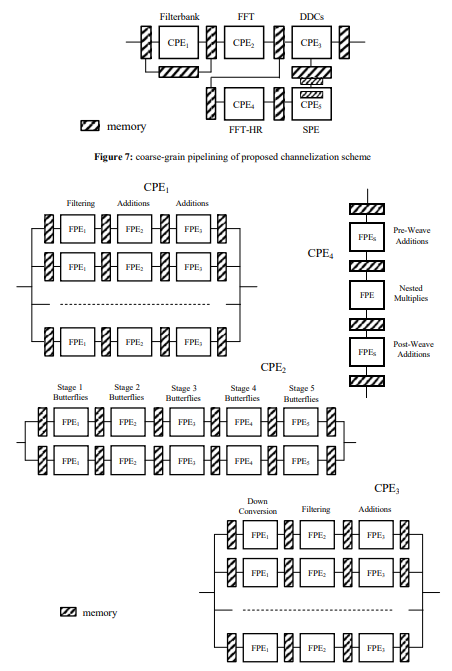
Figure 8: fine-grain pipelining of coarse-grain PEs required by channelization schemeA

Operation of Polyphase Filter bank

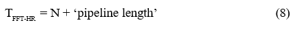
The components catered for by CPE1, as illustrated in Fig. 8, make up the polyphase filter bank, which may be implemented in the fashion of Jones [12] but with eight (rather than two) short, highly-parallel branch filters – each typically requiring just four to six fast multipliers and executing within a single clock cycle – running in parallel where each is operating upon an appropriately defined subset of the input data stream that is contained within its own memory [11]. This enables a new set of polyphase filtering outputs to be produced every

clock cycles, where ‘L’ is the number of filter taps per branch, which is well within the allotted update time. A few stages of additions are required at the output of the short branch filters in order to complete the production of the filtered outputs. A double buffering scheme may be devised for the branch filters which would ensure that whilst one buffer is being updated with new data, the data from the other is being fed into and processed by the branch filters. The operation of the two buffers, each comprising a bank of eight memories – one memory for each branch filter – would need to alternate every N/4 clock cycles.

Operation of Complex-Data FFT

The components catered for by CPE2, as illustrated in Fig. 8, make up the complex-data FFT, which may be implemented as a computational pipeline where each stage of the pipeline, for the case of a radix-4 FFT, carries out the execution of N/4 butterflies [2,3]. The availability of two highly-parallel radix-4 butterfly processors running in parallel – each typically requiring 16 fast multipliers and executing within a single clock cycle – for each of the log4N stages of the FFT will thus enable a new output set to be produced every

clock cycles, again well within the allotted update time. The complex-data FFT is illustrated in Fig. 8 by means of a 1024-point radix-4 algorithm, so that five stages of butterflies are required for its pipelined computation. Double-buffered memory is placed between successive stages, with each buffer comprising a bank of eight memories to ensure that the butterfly processors can operate at the required speed.

It should be noted that the overlapping of the input data segments to the polyphase filters results in an additional timing constraint in that for synchronisation of the two FFTs being simultaneously performed via the complex-data FFT – namely, that required by the PDFT module and that required by the row-DFT stage of the high-resolution FFT module – it is necessary that M×N windowed samples are made available to the FFT every M×N/4 clock cycles. Given that it takes M×N clock cycles to move this amount of data into the buffer, it is necessary that the data stored by the two buffers (as required for double buffering) should also be 75% overlapped.

This may be achieved with each buffer being partitioned into a bank of four memories, as already seen in Fig. 6, with the operation of the two buffers alternating every M×N/4 clock cycles. The entire set of M×N input samples must be available in the required buffer before the processing can begin, however, as each set of ‘N’ samples for input to a given large N-point FFT will come – according to the index mapping – from different parts of the data buffer. As a result of the overlapping of the input data, the high resolution FFT spectra are produced at four times that obtained with contiguous data sets, so that delays in detecting changes to the signal environment may be kept to a minimum.

Operation of DDC Units

The components catered for by CPE3, as illustrated in Fig. 8, make up the DDC module, where each unit is carried out in three (or more) stages with the first stage performing the frequency shifting of the signals of interest, the second stage the application of the filtering coefficients and the remaining stage(s) the summing of the results. Given that the channelization process reduces the sampling frequency out of the PDFT module by a factor of N/4, when compared to the initial system sampling frequency, the computational demands placed upon each DDC unit will not be great. In fact, for each N/4 new samples input to the PDFT module, there will be just one sample being input to each DDC unit that has been assigned to a PDFT channel.

The situation is further simplified by noting that the sampling frequency is consistent with the maximum signal bandwidth of interest, so that for the case where the signal bandwidth is significantly less than the channel bandwidth, a further reduction in the sampling frequency out of the DDC unit may be obtained.

Operation of Column-DFT Stage of High-Resolution FFT

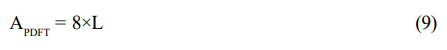
The components catered for by CPE4, as illustrated in Fig. 8, make up the column-DFT stage of the high-resolution FFT, which involves the computation of ‘N’ short M-point FFTs. The entire set of M×N input samples must be available in the required buffer – containing the appropriate unpacked outputs from the complex-data FFT – before the processing can begin, however, as each set of ‘M’ samples for input to a given small M-point FFT will come – according to the index mapping – from different parts of the data buffer.

The short M-point FFTs may be straightforwardly pipelined, however, with a small number of pre-weave addition stages being followed by a single nested point-wise multiplication stage which is in turn followed by a small number of post-weave addition stages. A single, maximally parallel implementation of the M-point FFT, able to produce all ‘M’ outputs within a single clock cycle, would enable a new set of column-DFT outputs to be produced every

clock cycles, which for M > 4 and N >> M, is within the allotted update time (for the high-resolution FFT) of M×N/4 clock cycles. Double buffering is again used to enable one completed data set to be processed whilst the other is being updated with each buffer being partitioned into a bank of ‘M’ memories.

Remaining Components

The remaining components, namely those of CPE5, carry out the additional tasks required by the SPE module concerning the centre frequency and bandwidth estimation of each signal of interest followed by the selection of the channels of interest – namely, those PDFT channels that contain in their entirety the signals of interest. The algorithms required for carrying out these functions, however, will not possess the regularity of those based upon the FFT and the FIR filter, although one would not expect the computational demands, in view of the comparatively low channel sampling frequency, to be prohibitive.

Complexity Considerations

To assess the space complexity of the proposed channelization scheme it is necessary to consider both the arithmetic requirement and the memory requirement. This is now carried out, but only for the main system components, as the additional complexity associated with the low-rate SPE and DDC modules will be very much dependent upon the algorithms used, the rate at which the SPE information is to be updated and the number of signals needing to be processed (and signal bandwidths catered for) by the DDC module.

Arithmetic Requirement

The arithmetic requirement is first assessed, at least in terms of fast multipliers, for the main system components. In order to meet the timing constraints discussed in the previous section, the polyphase filtering carried out by the PDFT module needs

fast multipliers – note that a branch filter of length L = 4 has proved to be adequate for achieving good channel filtering performance, at least for the case of a 1024-branch PDFT, with respect to both the pass-band and stop-band regions. The complex-data FFT needs

fast multipliers, whilst the column-DFT stage of the high- resolution FFT module, when implemented as a single short computational pipeline, needs

fast multipliers, where ‘AFFTM’ is the number of fast multipliers required for the maximally parallel implementation of the short M point FFT. For the case where ‘M’ has a value of seven, for example, the corresponding 7- point complex-data FFT may be carried out at the cost of just 16 real multiplications so that ‘A_FFT-HR’ would also equate to 16 fast multipliers.

The total arithmetic complexity, at least for the components

Memory Requirement

The memory requirement for the proposed channelization scheme, including that for the storage of pre-computed filter coefficients, twiddle factors and index mappings in suitably defined LUTs, may be broken down into three components:

a) the pre-FFT processing will require a minimum storage, in words, of:

      – 2×N/4 for double buffering of new PDFT input data,

      – N×L for internal PDFT data storage,

     – 2×M×N for double buffering of high-resolution FFT input data,

      – N×L for polyphase filter coefficients

      – M×N for high-resolution FFT window coefficients;

b) the complex-data FFT processing, assuming for the purposes of illustration a radix-4 algorithm, will require a minimum storage, in words, of: 

     – 2×2×N for double buffering of low-resolution FFT input data,

     – log4N×2×2×N words for internal multi-stage FFT data storage,

     – 0.25×N for low-resolution FFT twiddle factors

     – 2 × 2 × N for double buffering of low-resolution FFT output data;

c) the post-FFT processing will require a minimum storage, in words, of:

    – 2×2×M×N for double buffering of high-resolution FFT input data,

    – M×N for high-resolution FFT input mapping,

    – M×N for high-resolution FFT output mapping

    – 2×M×N for double buffering of high-resolution FFT output data.

Thus, the total memory requirement, at least for the main components considered, may be expressed as

words, this figure taking account of the double buffering requirements of the various interconnecting components needed for meeting the timing constraints discussed in the previous section. Note, however, that the two index mappings required for the high-resolution FFT module could also be generated ‘on- the-fly’ – rather than accessed via a LUT – as is usually done with the conventional digit-reversal indexing techniques used by the more familiar fixed-radix FFT algorithms [2,3].

Sizing for Large Hypothetical System

Thus, for the case of a large channelization problem involving the generation of 512 wide bandwidth PDFT channels (i.e. for N = 1024) and the construction of a 7K-point high-resolution FFT (i.e. for M = 7) for the guidance of the subsequent DDC units, the space complexity – apart from that required by the SPE and DDC modules – assuming a value for ‘L’ of 4, may be approximated by

Kwords, for the memory requirement. With large systems such as this, the relatively low channel sampling frequency (which is just a small fraction of the initial system sampling frequency) suggests that a small amount of computing hardware could be shared over many channels – that is, shared by many DDC units – so as to minimize the requirement for additional resources by the SPE and DDC modules.

Summary and Conclusions

There are two standard approaches to the problem of wideband signal channelization, namely those based upon the use of a DDC unit and those based upon the use of a PDFT. There are clear advantages and disadvantages with both approaches, however, in that: a) with the DDC approach, optimal performance and flexibility is obtained but at the expense of a heavy computational load; whereas b) with the PDFT approach, a sub-optimal and less flexible performance is obtained but at a greatly reduced computational cost through the exploitation of a suitably defined FFT routine.

The research described in this paper has therefore sought to produce an intelligent channelizer which possesses a flexible design able to exploit the merits of both approaches for the case where the input data comprises real-valued samples. The two key design features have involved: a) the optimal setting of the PDFT parameters to ensure that for every signal of interest there is at least one channel within which the signal is completely contained; and b) the simultaneous computation of two real-data FFTs: the first as required by the PDFT and the second, a high- resolution FFT with ×4 update rate, that is able to accurately direct the application of the low-rate DDC units via the SPE module to the relevant PDFT channel outputs.

The result is a hybrid system that is able to produce channelized signals to the same quality as would be obtained with a purely DDC-based system, but at a computational cost on a par with a purely PDFT-based system. The reduced complexity offers the promise, when implemented in hardware, of an attractive resource-efficient solution with a low SWAP requirement.

References

1. Harris, F. J. (2022). Multirate signal processing for communication systems. CRC Press.
2. Oppenheim, A. V. (1999). Discrete-time signal processing. Pearson Education India.
3. Rabiner, L. R., & Gold, B. (1975). Theory and application of digital signal processing. Englewood Cliffs: Prentice-Hall.
4. Crochiere, R. E., & Rabiner, L. R. (1983). Multirate digital signal processing. Englewood Cliffs, NJ: Prentice- hall.
5. Vaidyanathan, P.P. (1993). Multirate systems and filter banks. Prentice-Hall.
6. Jacobsen, E., & Kootsookos, P. (2007). Fast, accurate frequency estimators. IEEE Signal Processing Magazine, 24(3), 123-125.
7. Good, I. J. (1958). The interaction algorithm and practical Fourier analysis. Journal of the Royal Statistical Society Series B: Statistical Methodology, 20(2), 361-372.
8. Winograd, S. (1978). On computing the discrete Fourier transform. Mathematics of Computation, 32(141), 175-199.
9. Cooley, J. W., & Tukey, J. W. (1965). An algorithm for the machine calculation of complex Fourier series. Mathematics of Computation, 19(90), 297-301.
10. Akl, S. G. (1989). The design and analysis of parallel algorithms. Prentice-Hall.
11. Maxfield, C. (2004). The design warrior's guide to FPGAs: devices, tools and flows. Elsevier.
12. Jones, K. J. (2013). Resourceâ?ÂÃÂ?efficient and scalable solution to problem of realâ?ÂÃÂ?data polyphase discrete Fourier transform channelization with rational overâ?ÂÃÂ?sampling factor. IET Signal Processing, 7(4), 296-305.
13. Burrus, C. (1977). Index mappings for multidimensional formulation of the DFT and convolution. IEEE Transactions on Acoustics, Speech, and Signal Processing, 25(3), 239- 242.
14. McClellen, J. H., & Rader, C. M. (1979). Number theory in digital signal processing. Prentice Hall.
15. Niven, I., Zuckerman, H. S., & Montgomery, H. L. (1991). An introduction to the theory of numbers. John Wiley & Sons.

Appendix

2-D Formulations of DFT

The mapping of one-dimensional (1-D) arrays into multi- dimensional (m-D) arrays provides the basis for most of the existing FFT algorithms. These mappings need to be both unique and cyclic in every dimension [13] to ensure that: 1) the original DFT can be recovered in its correct form; and 2) the correct periodicities are obtained for each of the small DFTs that constitute the m-D form. Mappings will now be briefly described for the conversion of a 1-D DFT to a separable 2-D DFT, as this is the formulation of interest in this paper.

Consider firstly the index transformations given by the linear forms:

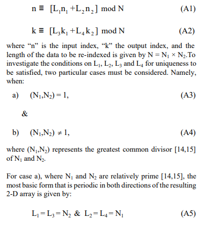
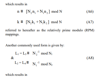
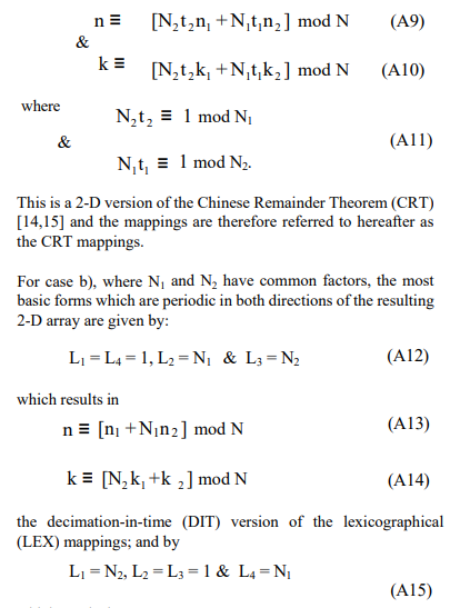
Applying the 2-D RPM and CRT mappings to the direct computation of the DFT, it is now seen how a 1-D DFT of composite length may be expressed in 2-D form, and vice versa, so that the computation of the respective 1-D and 2-D DFTs are essentially equivalent, one being simply derivable from the other. Application of the LEX mappings, as used by Cooley and Tukey [9], to the 1-D DFT is also considered, whereby a 2-D form is again achieved, although in this instance it does not correspond to a true separable 2-D DFT because of the resulting twiddle factor requirement. Factors N1 and N2 have common factors, the decomposition corresponds to the CFA, whilst when they are relatively prime, it corresponds to the PFA.

Suppose the length N of a 1-D DFT can be written as:

    N = N₁ ´ N₂                                                                              (A18)

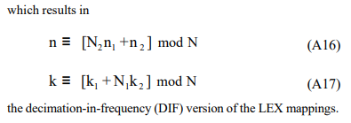
where N₁ and N₂ are arbitrary factors, with or without common factors. Then a sufficient pair of mappings, for the 1-D to 2-D transformation, may be given by the DIF version of the LEX mappings (as described by Eqtns. A16 and A17), enabling the DFT to be written as:

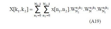
where k₁ = 0,1,…,N1-1 and k₂ = 0,1,…,N2-1, with W_N, WN₁ and WN₂ the primitive Nth, N1th and N2th complex roots of unity, 2 respectively.

The expression of Eqtn. A19 reduces the N-point DFT, for the two- factor case of interest, to an essentially three-stage process: a partial-DFT, followed by a point-wise matrix multiplication to account for the twiddle factors, followed by a second partial DFT. The only difference, therefore, between this formulation and that of a true separable 2-D DFT, is the presence of the twiddle factors, and it is now seen how, by appropriate choice of N and its factors, the twiddle factors can be eliminated.

Suppose that the factors N₁ and N₂ of Eqtn. A18 are relatively prime.

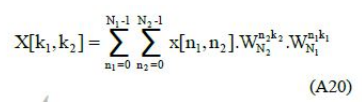
Then by applying the RPM mapping of Eqtn. A6 and the CRT mapping of Eqtn. A10 to the input and output data sequences, respectively, the DFT can be written as:

a true separable 2-D DFT, without twiddle factors, consisting of just the two partial-DFT processes. The intermediate data simply requires straightforward re-ordering, via the LEX mapping, prior to being input to the second partial-DFT stage. It should be noted, from this two-factor formulation, that only one of the two index mappings – and it can be for either input or output – actually needs to satisfy the CRT in order that a true 2-D DFT be obtained, although a true 2-D DFT is also obtained if both index mappings satisfy the CRT.