Analysis of selected algorithms for the classification of space objects?

Introduction

In modern astronomy, increasing number of data is becoming an ever-growing problem and opportunity. Formulation and validation of many theories require scientists to go through huge databases, which have become impossible to do by hand. At the same time, increasing capabilities of earth-based observatories and space telescopes are providing us with many sky surveys containing petabytes of quality data [1,2]. This data-intensive situation encourages the investigation of new methodologies, big data tools and techniques, therefore providing a great environment for astro-informatics development [3].

Machine learning has a significant impact on this new reality [4- 6]. It provides many tools that can be used to swiftly classify huge amounts of data, which we will try to explore in this paper. We will go through algorithms such as Decision Tree, Naive Bayes and K-Nearest Neighbors and analyze their accuracy to distinguish between different objects [7-9].

Methodology

In the beginning, we will need to transform our data into aconvenient form. In the case of the non-numerical data, we will simply map it to one by associating separate numbers for each value. On the other hand, numerical data will be rescaled using min-max normalization.

We will compare performance of different algorithms, given the task of classification of stellar objects. For the comparison, we have chosen:

• KNN (K-Nearest Neighbors) classification.

• Decision tree model.

• Naive Bayes.

Mathematical Model for K-Nearest Neighbors (K-NN)

If we assume we have a training dataset consisting of N data points:

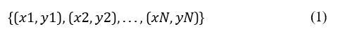
where x_i is the feature vector for the i-th point, and y_i is the class label (for classification) or value (for regression).

Then we can calculate a distance metric, typically using the Euclidean distance d between two points x and z defined as

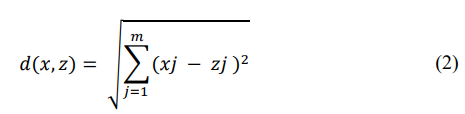
where x and z are feature vectors of dimension m.

To classify a new point x we compute the distances between x and all points in the training set, then select K nearest neighbors and assign a class label based on the majority.

The parameter K is a crucial hyperparameter in the KNN algorithm. A small K can lead to overfitting, while a large K can lead to underfitting. The optimal value of K is often selected usingcross-validation methods.

Algorithm 1: KNN Algorithm

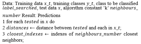
4 labels ←classes of closest neighbors;

5 result← dominating label in labels

6 Add result to prediction list;

7 Create data structure with predictions, by choosing indexes of the test data; return Predictions

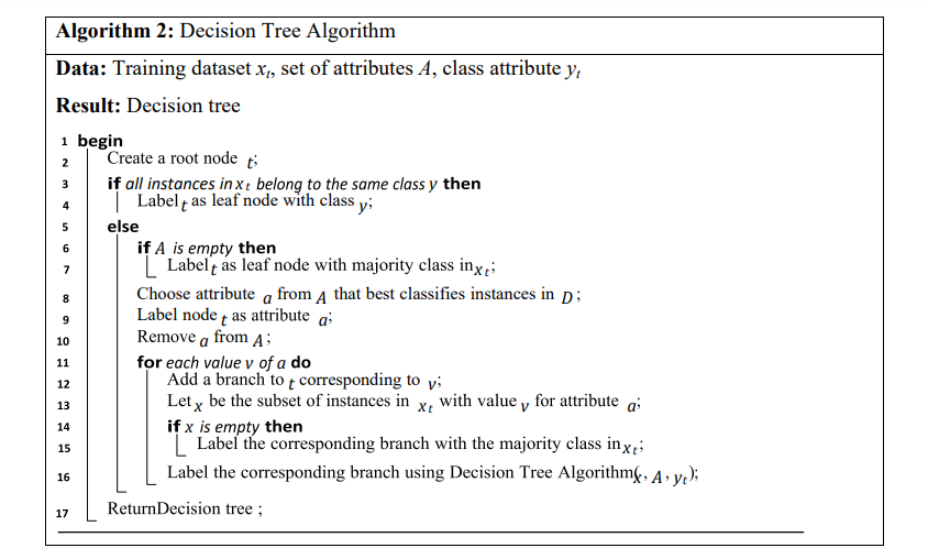
Mathematical Model for Decision Tree

If we assume we have a training dataset consisting of N data points

where x_i is the feature vector for the i-th point, and y_i is the classlabel (for classification) or value (for regression). Then a decision tree is a tree-like model where internal nodes represents a test on a feature, branches represents outcomes of those tests and leaf node represents a class label.

To build a decision tree, we recursively split the data at each node. The choice of split is based on a criterion that maximizes the separation of the classes or reduces the prediction error.

Common criteria include:

Gini Index:

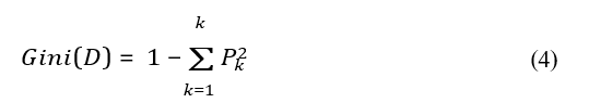
where p_k is the proportion of instances of class k in the dataset D.

Information Gain:

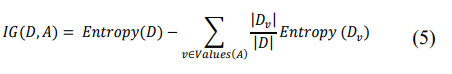
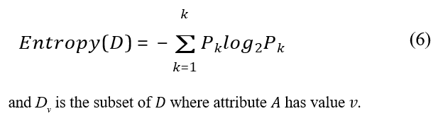
where Entropy(D) is given by:

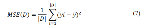
Mean Squared Error (MSE):

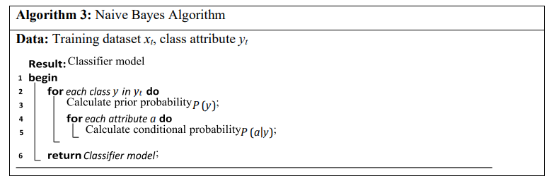
Mathematical Model for Naive Bayes

Assume we have a training dataset consisting of N data points:

where x_i = (x_i1,x_i2,...,x_im) is the feature vector for the i-th point, and y_i is the class label from a set of classes {C₁,C₂,...,C_K}.

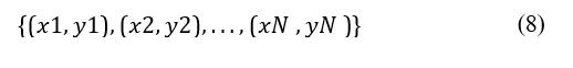
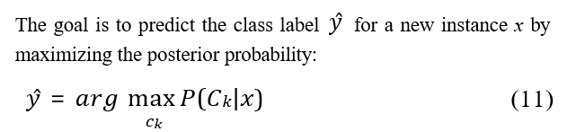
The Naive Bayes algorithm is based on Bayes’ Theorem:

where: P(C_k | x) is the posterior probability of class C_k given featurevector x, P(x | C_k) is the likelihood of feature vector x given class C_k, P(C_k) is the prior probability of class C_k, P(x) is the evidence or marginal likelihood of feature vector x.

 The "naive" assumption is that the features are conditionally independent given the class label:

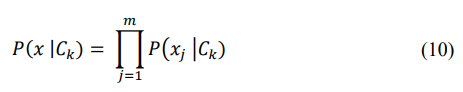
Using Bayes’ Theorem and the naive assumption, we can write:

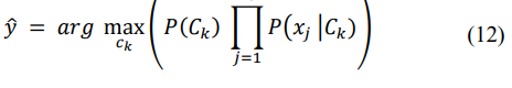
The probabilities P(C_k) and P(x_j | C_k) need to be estimated from the training data and the prior probability of class C_k is estimated as:

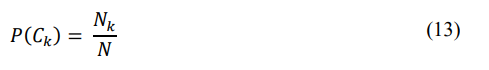
where N_k is the number of instances in class C_k. For continuous features, a common approach is to assume a Gaussian distribution:

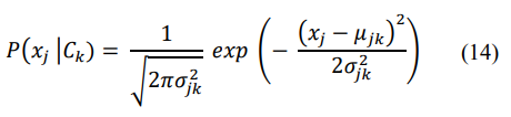
where µ_jk and σ_jk²are the mean and variance of the feature x_j for class C_k.

Additionally, we will look for the best number of neighbours for KNN classifier. We will use a few libraries to handle our operations: Sklearn - will provide us with algorithm implementations, saving us a lot of time and ensuring we will be able to go through relatively big databases in reasonable time [10]. Pandas - will provide us with data structure (DataFrame) [11]. Seaborn and Matplotlib - will be used for visualizations, graphs, etc [12,13].

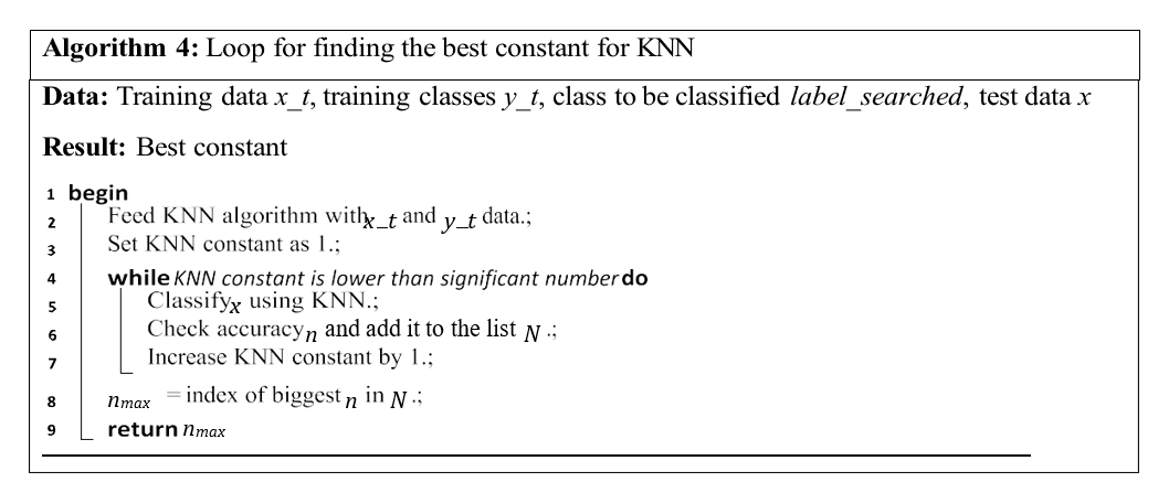
In order to find the best constant for KNN, we will launch classification in a simple loop, looking for the best solution. Generally speaking, when this number will increase our accuracy should decrease, therefore this approach is reasonable and should not take too much time.

In the end, we present the confusion matrix for each of our solutions, and we will consider only two metrics:

• Accuracy (Equation 15) - to measure how many correct classifications we get.

• False categorization - in order to check if any of the classes are more often confused with others.

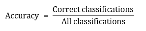
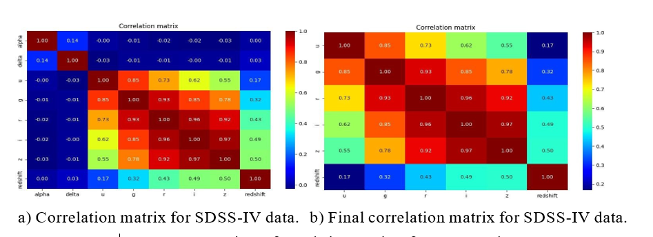
Figure 1: Comparison of correlation matrices for SDSS-IV data

Experiments

For our dataset, we have chosen data from Sloan Digital Sky Survey DR17 [14,15]. Which was the fourth phase of the Sloan Digital Sky Survey (we will call it SDSS-IV from now on). It contains 100000 observations, each containing (qouting [16]):

• obj_ID = Object Identifier, the unique value that identifies the object in the image catalogue used by the CAS

• alpha = Right Ascension angle (at J2000 epoch)

• delta = Declination angle (at J2000 epoch)

• u = Ultraviolet filter in the photometric system

• g = Green filter in the photometric system

• r = Red filter in the photometric system

• i = Near Infrared filter in the photometric system

• z = Infrared filter in the photometric system

• run_ID = Run Number used to identify the specific scan

• rereun_ID = Rerun Number to specify how the image was processed

• cam_col = Camera column to identify the scanline within the run

• field_ID = Field number to identify each field

• spec_obj_ID = Unique ID used for optical spectroscopic objects (this means that 2 different observations with the same spec_obj_ ID must share the output class)

• class = object class (galaxy, star or quasar object)

• redshift = redshift value based on the increase in wavelength

• plate = plate ID, identifies each plate in SDSS

• MJD = Modified Julian Date, used to indicate when a given piece of SDSS data was taken

• fiber_ID = fiber ID that identifies the fiber that pointed the light at the focal plane in each observation

a.)Histograms for all normalized data, excluding redshift.      b) Histogram for normalised redshift. 

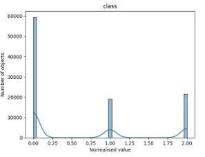
         c) Number of different objects (0 - galaxies, 1 - QSOs, 2 - stars).

                                         Figure 2: Various histograms showing data distributions and object counts.

Some of that information will not be used for our classification, as they are contained in SDSS-IV for cataloguing purposes (such as object identifiers). We will focus on: coordinates alpha and delta; data from filtered channels u, g, r, i and z; class, which is the aim of our classification efforts.

After mapping and normalising our data in ultraviolet, green and infrared presented strange pattern, where basically all data is accumulated near value 1.0. Upon further inspection it turns out that one of the observed objects have some abnormal values (equals to -9999), we will remove it from our dataset and then proceed.

Now we will have a look at the correlation matrix (figure 1a) and address some of the relations:

• Coordinates have neutral relations with all the other data.

• Ultraviolet and green relation- green light is a part of spectrum of many stars similar to the Sun (G-type main-sequence stars). Those stars also happens to emit significant part of their radiation as ultraviolet. An additional effect, that can also explain moderate relation with infrared and near infrared light is absorption and re- emission of different by interstellar gas, which then re-emits in those wavelengths (heat radiation) [17].

• Infrared, near-infrared and red data have strong relation - red stars are typically colder, but they still emit a lot of infrared radiation. Additional factor - absorption and re-emission of light was mentioned above.

• Moderate relation of red, near infrared and infrared light with redshift can by explained by many objects detected as red having their colour shifted due to phenomenons as Doppler effect. This relation might be absent from other detectors, as light of stars different from infrared might have been cut off by stardust or shifted strong enough to not be detected at all [17].

In general, it is easy to notice strong relations with red and infrared light. This phenomenon might be related to extinction of light in the space, which is more explicit for shorter wavelengths.

The coordinates of our objects are mostly related to each other (but it is still very weak relation). It also has a pure neutral relation with most of the data from detectors, therefore we are going to drop this one. Our final correlation matrix is shown for the sake of clarity in figure 1b.

Additionally, we will provide histograms for SDSS-IV data, we will plot them on to one histogram, excluding redshift, which will be shown separately for clarity (figures 2a and 2b). We will also have a look at a number of each of the individual objects in our data (figure 2c) we can notice significant dominance of galaxies. Galaxies and quasars are similar in number, with a small margin for stars.

We will split our data with at train and test set with ratio of 0.2. After running the calculation mentioned in chapter before, we get:

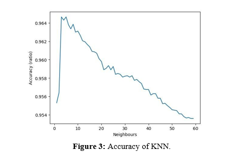
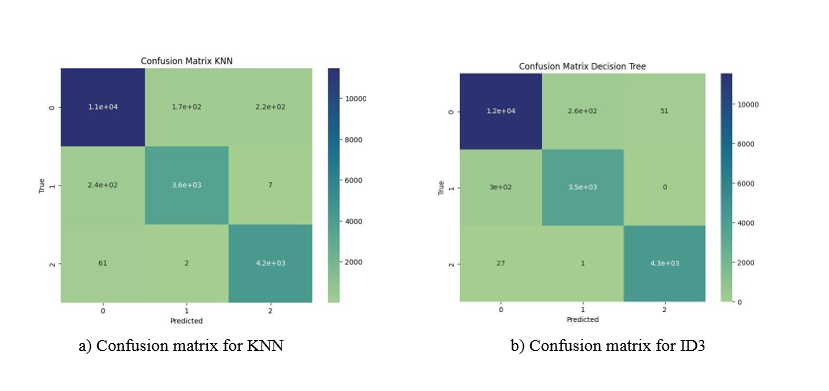
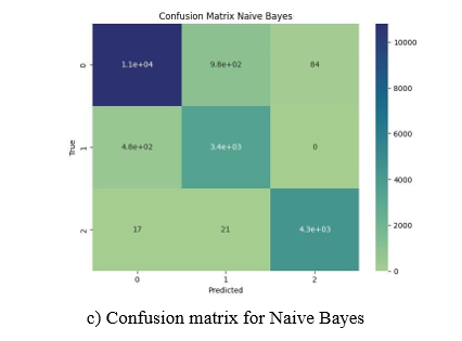
Figure 4: Comparison of confusion matrices for KNN, ID3, and Naive Bayes Algorithms (0 - galaxies, 1 - QSOs, 2 - stars).

• For KNN we get 96.465% accuracy, which was best for numbers of neighbors equal to 3 as shown in figure 3 with confusion matrix as in figure 4a.

• Decision tree have achieved 96.78% accuracy (confusion matrix in figure 4b).

• Naive Bayes have achieved the lowest accuracy of 92.11% (confusion matrix in figure 4c)

Conclusion

Behavior of KNN accuracy was, as expected, decreasing with relation to its constant. On the other hand, all the analyzed algorithms achieved good accuracy (above 90%). Bayes algorithms turned out to have had some problems distinguishing between galaxies and quasars (almost 1000 wrongly classified galaxies), although two others algorithms also struggled there. KNN seems to deal the best with this problem, recognizing even so slightly more QSO objects than others but have more mismatches, recognizing some of the galaxies as stars. None of the algorithms have any problems recognizing stars and rarely ever mismatches them [18].

References

1. Becker, B., Vaccari, M., Prescott, M., & Grobler, T. (2021). CNN architecture comparison for radio galaxy classification. Monthly Notices of the Royal Astronomical Society, 503(2), 1828-1846.
2. Iess, A., Cuoco, E., Morawski, F., Nicolaou, C., & Lahav,O. (2023). LSTM and CNN application for core-collapse supernova search in gravitational wave real data. Astronomy & Astrophysics, 669, A42.
3. Zhang, Y., & Zhao, Y. (2015). Astronomy in the big data era.Data Science Journal, 14, 11-11.
4. Xu, L., Wang, J., Li, X., Cai, F., Tao, Y., & Gulliver, T. A. (2021). Performance analysis and prediction for mobileinternet-of-things (IoT) networks: a CNN approach. IEEE Internet of Things Journal, 8(17), 13355-13366.
5. Wozniak, M., Szczotka, J., Sikora, A., & Zielonka, A. (2024). Fuzzy logic type-2 intelligent moisture control system. Expert Systems with Applications, 238, 121581.
6. Polap, D., Kesik, K., Winnicka, A., & Wozniak, M. (2020). Strengthening the perception of the virtual worlds in a virtual reality environment. ISA transactions, 102, 397-406.
7. Wozniak, M., & Polap, D. (2020). Soft trees with neural components as image-processing technique for archeological excavations. Personal and Ubiquitous Computing, 24(3), 363-375.
8. Wickramasinghe, I., & Kalutarage, H. (2021). Naive Bayes: applications, variations and vulnerabilities: a review of literature with code snippets for implementation. Soft Computing, 25(3), 2277-2293.
9. Ukey, N., Yang, Z., Li, B., Zhang, G., Hu, Y., & Zhang, W. (2023). Survey on exact knn queries over high-dimensional data space. Sensors, 23(2), 629.
10. Package of scikit-learn. 2024. Accessed: 2024-05-17.
11. Pandas library, 2024. Accessed: 2024-05-17.
12. Seaborn library, 2024. Accessed: 2024-05-17.
13. Matplotlib library, 2023. Accessed: 2024-05-17.
14. Original source of data release 17 from sloan digital sky survey, 2022. Accessed: 2024-05-18.
15. Source of our data at kaggle.com, 2022. Accessed: 2024-03- 29.
16. Fedesoriano, Stellar classification dataset - sdss17, 2022. Retrieved May 18, 2024.
17. Article about infrared imaging, 2024. Accessed: 2024-05-18.
18. Jedrzejczyk, R., & Kleczek, K. Analysis of selected algorithms for the classification of space objects.