Towards Sustainable Viable Economic Development: Leveraging Heat Exchange Networks and The Return on Incremental Investment Metric

Introduction

Considerable research effort is currently underway to reducereliance on conventional fossil-based fuels and utilize renewable energy sources, leading to energy savings and reduced environmental impact. In this respect, industrial heat integration, through pinch analysis, plays a crucial role in mitigating climate change by reducing energy consumption, fossil fuel usage, and greenhouse gas emissions. The breakthrough of the concept of pinch technology in optimal HEN design was introduced by Linnhoff and Flower and Linnhoff and Hindmarsh [1,2]. Since its introduction, pinch technology has been extensively applied in engineering and other fields. The pioneering work of El-Halwagi and Manousiouthakisand El-Halwagisaw the introduction of mass exchange networks to parallel theconcepts of HENs [3,4]. Considerable research was carried out on the problem of reducing the usage of external sources of heating and/or cooling utilities [5-9]. Several reviews were published on the subject [10]. HENs enhance sustainability of fuel resources by optimizing energy usage within industrial processes. This can contribute to a more sustainable and efficient use of available fuel resources. Furthermore, recovering and reusing waste heat reduces plant operating expenses by reducing the need for additional fresh energy inputs.Nonetheless, there is scarcity in the literature on theeconomic techniques for rigorous economic analysis for the evaluation of emerging energy-efficient technologies. Needless to say, any new technology must be economically viable to be accepted and commercialized as an energy source to meet market demand.For green grass projects involving heat networks, the design stage should involve the consideration of the economics of heat integration. The ensuing capital costs associated with the addition of new equipment for the purpose of reducing external utility operating costs must realize an acceptable return on investment.

The contribution of the research problem in this work involves the presentation and analysis of the novel concept of Return on Incremental Investment (ROII). The basic idea is that when considering an energy-saving technology that involves capital expenditure, such as proposing new and more efficient equipment as an alternative or replacement for less efficient equipment, it is imperative to ensure the economic viability of this investment endeavourby evaluating the resulting energy savings as a return on the incremental investment. The ROII metric is defined as the percentage of the ratio of annual savings in energy to the ensuing increase in capital expenditure in terms of depreciable cost of equipment. The technique is applied to a case study.The case study outlined in this study is the heat network in a simplified chemical processing facility shown in Figure1 below adapted from El Halwagi [4]. The process involves two adiabatic reactors, a scrubber, a separation network, two heaters, two coolers, and a flash column.The emphasis in this study is on the heat network involved rather than the processing operations involved. It is important to note that the application of the proposed economic technique is not limited to chemical processing plants, but ratherto any industrial venture where new equipmentor technologyis intended to replace obsolete equipment or technology.In this contribution, a step-by-step procedure is outlined in the methodology section from conception to the final calculation of ROII.

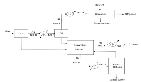
Figure 1: Simplified Chemical Facility El-Halwagi [4]

Methodology

This study is a conceptual presentation of a novel economic evaluation method for the project of replacement of an obsolete technology with a new more efficient one. Such a replacement usually involves capital expenditure in terms of the incremental cost due to the difference between the cost of the new and old equipment. The ensuing savings in operating costs (e.g., steam and cooling water costs in this case study)should represent an acceptable economic justification for the incremental capital costs. The case study in this work involves the replacement of a heat network in a green grass simplified chemicalfacility involving, heating and cooling units, with a new heat exchange network (HEN). The existing heat network is supplied with its requirements of steam and cooling water, at a cost, from external sources. The objective of this replacement is to expediently reduce the cost of energy consumption by exchanging heat between hot and cold streams.

The first step in the technique involves the extraction of thermodynamic data from the hot and cold streams. An approach temperature is assumed. The heat integration algebraic method is then carried out to determine thepinch point(s) as well as the minimum heating and cooling requirements of the HEN. This step is called the targeting stage and is carried outaccording to the following steps, El-Halwagi: A temperature interval table (TID) is constructed to establish the feasible heat exchange rates within each temperature interval on the basis of the specified approach temperature [4]. Heat balances are carried out over each interval and a cascade diagram is constructed from the TID data. The most negative heat residual load marks the most infeasible interval as well as the location of the pinch point. A revised cascade diagram is next built by adding the most negative heat residual to the top interval to remove all infeasibilities. This heat load represents the minimum heating requirement. The minimum cooling requirement is the heat load leaving the bottom interval the heat loads of the heat exchangers are determined by carrying energy balances round each feasible heat exchanger. The heat transfer area of each heat exchanger is calculated through the design equation Q = UAT, where Q is the heat load, U the overall heat transfer coefficient, and T is the temperature difference between the hot and cold fluids. The cost of the heaters, coolers, and heat exchangers are calculated on the basis of the heat transfer areas. The installed cost of each heat exchanger was estimated on the basis of $ 500 per square meter[9] . The currency units are US dollars throughout the study. The installed costs of the coolers and heaters were estimated at 50% of the cost of a comparable heat exchanger with the same heat transfer area and material of construction. The difference in costs due to sizes was corrected using the six tenth rule. The material of construction is carbon steel for all equipment.Utility costs for the two cases were calculated on the basis of cooling water cost at 0.354 ($/GJ) and steam cost at 6.08 ($/GJ) as reported by the software application CAPCOST.

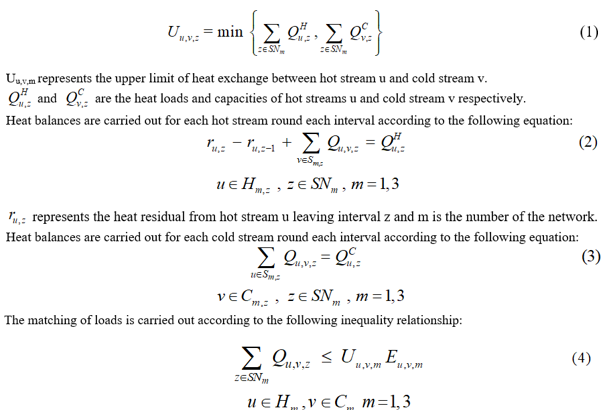
The optimization problem of determining the minimum number of heat exchangers was carried out byimplementing the linear programming technique using the LINGO software application. The LINGO code and therelevant solution are presented in the appendix. Stream matching is implemented within each subnetwork separately to avoid cross matching over pinch borders. Matching of streams across pinch line would result in passing heat through a pinch point which would result in three negative results: increasing heating requirements; increasing cooling requirements; and reducing heat exchange in the overlapping heat exchange range El-Halwagi [4]. Stream matching of each couple of streams involves the determination of the upper limit of heat exchange between the heat load of the hot stream and the capacity of the cold stream according to the constraint relationship El-Halwagi:

The last stage in this project is the economic evaluation. The incremental capital cost is determined by computing the difference between the depreciable costs of all the heat exchangers and the depreciable costs of all the heaters and coolers. A service life time of ten years is assumed for all equipment. The reduction of utility costs is the difference between the original utility costs and the new utility costs. The optimization stage in this study involves the determination of the minimum capital cost, represented by the minimum number of heat exchangers, that meets the minimum operating costs already realized in the targeting stage implemented by the algebraic method through the revised cascade diagram. The total number of heat exchangers is the sum of all possible matching of streams in the three subnetworks. The symbol Eij is used to refer to the heat exchanger which exchanges heat between hot stream (i) and cold stream (j). The objective function to be minimized is thus:

Minimize = ∑E112 + E122 + E212 + E222                (5)

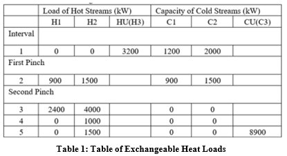
The software LINGO is used to run the linear programming optimization program. Table 1belowshows the exchangeable heat loads data used for program execution. Stream matchings are implemented within individual subnetworks only. In each stream matching the upper bound of the heat stream load and the cold stream capacity is taken as the exchangeable load.

The ROII is calculated as the result of the division of the savings in utility costs by the incremental capital cost.

ROII = Savings in Utility Costs / Incremental Capital Cost (5)

Results and Discussion

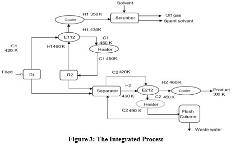
In addition to the objective function equation, the LINGO program involves heat balances for H1, heat balances for H2, heat balance for steam utility HU (H3), heat balances for C1, heat balances for C2, heat balance for cooling water utility CU (C3), matching of loads equations, non-negativity constraints, and declaration of binary integers El-Halwagi [4].The solution of the LINGO program indicates that the optimal configuration network requires the introduction of two heat exchangers out of the possible four cases in the objective function. In addition, two smaller heaters and two smaller coolers are needed to provide the utility loads needed to meet the balance of the minimum requirements specified in the revised cascade diagram. Figure 3 below shows the expedient placement of the two heat exchangers E112 and E222 and the smaller two heaters and two coolers in the integrated system. The annual utility costs, and capital expenditures are presented in tables 2, 3 ,4, and 5 below.

Annual cooling water cost for cooling streams H1 and H2 =

(3,300 + 8000) X 10-6 GW X 3600 X 7920 s/year X 0.354 $/GJ

Annual steam cost for heating streams C1 and C2

= (2,100 + 3500) X 10-6 GW X 3600 X 7920 s/year X 6.08 $/GJ

Figure 2: Steps for Project Implementation

The utility costs for the base case are shown in TABLE 2 below

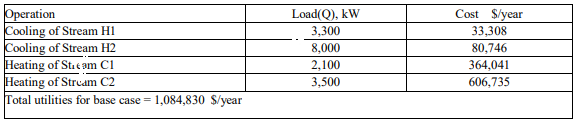
Table2: Annual Utility Costs for the Base Case

Similar calculations were carried out for the integrated case and the results are shown in TABLE 3 below.

                                                  Table 3: Annual Utility Costs for the Integrated Case

The heat transfer area of the heat exchangers was calculated from heat balances round the heatexchangers. The design equation used is:

Where Q is the heat load, U the overall heat transfer coefficient, and T is the temperature difference between the hot and cold fluids. The individual heat temperate difference above T is used rather than the log mean temperature difference (LMTD) because the log mean temperature differenceisusually used in heat exchanger design, analysis, and measurement of heat exchanger performance. The difference in accuracy between the two methods might be negligible when the temperature differences are small or when the fluids are nearly counter-current. The purchased costs of heaters and coolers in the base case are shown in Table 4 below.

                                             Table4:Purchased Costs of Heaters and Coolers in the Base Case 

The purchased costs of heat exchangers, heaters, and coolers in the integrated case is shown in Table 5 below.

                        Table 5:Purchased Costs of heat Exchangers, Heaters, and Coolers in the Integrated Case

The ROII is calculated as follows:

The base case investment = Purchased costs of base case two heaters and two coolers.

The integrated case investment = Purchased costs of two heat exchangers + Purchased costs of the new two heaters and two coolers.

Incremental capital investment = Integrated case capital investment - Base case capital investment

Annual Profits = Annual savings in utility costs + annual savings in depreciations costs (which are expected to be negative in value)

ROII = Annual profits / Incremental capital investment

Depreciation costs of equipment for the base case = 2,177,940 /10 =217,794 $/year

Total of utilities and equipment depreciation costs for base case =1,302,624 $/year

Depreciation costs of equipment for integrated case = 2,657,562/10 = 265,756 $/year

Total cost of utilities and equipment depreciation costs for integrated case = 986,860 $/year

Net annual savings in utility and equipment depreciation costs = 1,302,624 -986,860 = 315,764 $/year

Incrementalcapital =2,657,562 - 2,177,940= $ 479,937

Percentage return on incremental capital cost (ROII) = (315,764/479,622)*100 =65.8%

Sensitivity Analysis

Fuel costs have a significant impact on process economic performance in general and on thermal process integration in particular. Table 6 below shows the sensitivity of changes in utilities' costs (which are directly driven by fuel costs) on annual profits. Steam costs are by far the dominant utility cost component. An increase in utilities costs represents an increase in both versions of the projects under study and thus represent an increase in the difference of the utility costs between the two cases. In other words, an increase in utility costs improves the value of the ROII. For example, a 10% increase in utility costs would be reflected in a 10% increase in annual savings. The results of the calculations are as follows:

Net annual savings in utility and equipment depreciation costs =315,764 $/year

Annual savings in utility costs alone = 1,084,830 - 721,104 =363,726 $/year

Net cost in depreciation costs = 72,598 - 181,700 = - 47,962$/year

                                               Table 6:Effect of Increases in Utility Costs on ROII Metric

Table 6 above indicates that the profitability of the proposed integration in terms of the ROII metric is very sensitive to increases in utility costs which are directly impacted by increases in energy costs.

On the other hand, a decrease in energy costs reduces utility costs and subsequently the difference between the utility costs of the two cases under consideration. Such a situation reduces the economic incentive to implement thermal integration. Table 7 below assesses the effect of lower utility costs on process economic performance.

                                    Table7: Effect of Decreases in Utility Costs on ROII Metric

Table 7above indicates that there is an important threshold of minimum or cut off ROII (to be predetermined by plant manager) below which the project becomes economically untenable. Throughout the sensitivity analysis it is assumed that the equipment costs remain constant and do not fluctuate as does the utility costs.

Conclusion

The results of the study highlight the sensitivity of profits to utility costs which are driven directly by energy costs fluctuations. The impact of changes in capital costs also impact profitability but to a lesser extent because these effects are delayed and are not immediate. The estimation of equipment costs is critical to the assessment of project economicperformance. The economic viability is highly impacted by the cost of heat transfer equipment in terms of dollars per unit surface area as quoted from market suppliers. The equipment heat transfer area is critically sensitive to the assumed overall hear transfer coefficient (U).The cost of heat exchangers, heaters, and coolers should be obtained directly as quotations from manufacturers or venders. The project realizes a ROII of 65.8%. The steps outlined in this contribution would assist decision makers and researchers in arriving at logical actions based on informed opinions [11-14].

Nomenclature

Cpu Specific heat of hot stream u kJ/kgK

C pv Specific heat of hot stream v kJ/kgK

Eu v m, ,binary integer variable that takes the value of0when there is no match between streams u and v in SNm and takes the value of 1 when there is a match

fflow rate of cold stream (kg/s)

F flow rate of hot stream (kg/s )

HHu z,hot load in interval z

HCv z, cold capacity in interval z

NC number of process cold streams

NCU number of cooling utilities

NH number of process hot streams

NHU number of heating utilities

Qu v z, , heat exchanged from hot stream u to cold stream v in interval z

R1,R2 Reactors 1 and 2

rz residual heat leaving interval z

ru z, residual heat leaving interval z from hot stream u u index for hot streams

v index for cold streams

Uu v m, , upper bound on the exchangeable heat load between streams u and v in SNm

z temperature interval

Statements and Declarations

Funding

The authors declare that no funds, grants, or other support were received during the preparation of this manuscript

Competing interests

The authors have no competing interests to declare that are relevant to the content of this article. All authors certify that they have no affiliation with or involvement in any organization or entity with any financial interest in the subject matter or materials discussed in this manuscript. The authors have no financial or proprietary interests in any material discussed in this article.

Author contributions

All authorscontributed in a collaborative effort to the study conception and design. All authors contributed to the previous version of the manuscript.

Data Availability Declaration

The authors declare that any data supporting the findings in this study are available within the paper.

References

1. Linnhoff, B., & Flower, J. R. (1978). Synthesis of heat exchanger networks: I. Systematic generation of energy optimal networks. AIChE journal, 24(4), 633-642.
2. Linnhoff, B., & Hindmarsh, E. (1983). The pinch design method for heat exchanger networks. chemical engineering science, 38(5), 745-763.
3. El-Halwagi, M. M., & Manousiouthakis, V. (1989). Synthesis of mass exchange networks. AIChE Journal, 35(8), 1233-1244.
4. El-Halwagi, M. M. (2017). Sustainable design through process integration: fundamentals and applications to industrial pollution prevention, resource conservation, and profitability enhancement. Butterworth-Heinemann.
5. Klemes, J. K. (2011). Wan Alwi SR Review of Progress in Integration Technologies for Intensified and Sustainable Processes.
6. Chemical Engineering Research and Design, 89, 1271-1288.
7. Klemes, J. J., & Varbanov, P. S. (2012). Process Integration of Heat and Power Systems: A review. Applied Energy, 92(1), 297-313.
8. Klemes, J. J., Vanbnov, P. S.,Kravanja, Z. (2013).Recent Development in Process Integration. Chemical Engineering Research and Design”.
9. Klemes, J. J., & Pierucci, S. (2016). Sustainability Assessment of Process Integration: A review. Journal of Cleaner Production,133, 38-55.
10. Klemes, J.J., Wang, Q., Varbanov,, P.S., Zeng, M., Chin, H., Lal, N.S., Li, N., Wang,, B., Wang, X., Walmsley, T. (2020).Heat Transfer Enhansement, Intensification and Optimization in Heat Exchanger Network Retrofitting and Operation”. Renewable and Sustainable Energy Reviews.
11. Manan, Z.A., Mustafa, s., Shamsuddin, A.H., &Wan Alwi, S.R. (2016). Energy Integration and Optimization of Industrial ProcessesThrough Pinch Analysis: A Comprehensive Review. Energy Conversion and Management, 105, 821 – 842.
12. Ndeke, C. B., Adonis, M., & Almaktoof, A. (2024). Energy management strategy for a hybrid micro-grid system using renewableenergy. Discover Energy, 4(1), 1.
13. Riadi, I., Putra, Z. A., & Cahyono, H. (2021). Thermal integration analysis and improved configuration for multiple effect evaporatorsystem based on pinch analysis. Reaktor, 21(2), 74-93.
14. Wagialla, K. M., El-Halwagi, M. M., & Ponce-Ortega, J. M. (2012). An integrated approach to the optimization of in-plant wastewater interception with mass and property constraints. Clean Technologies and Environmental Policy, 14, 257-265.
15. Wagialla, K. M. (2012). Pinch-based and disjunctive optimization for process integration of wastewater interception with mass and property constraints. Clean Technologies and Environmental Policy, 14, 597-608.

Appendix

LINGO Code:

Min = E112+E122+E212+E222;

!Heat balance for hot stream H1;

r12+Q112+Q122=900;

r13-r12=2400; r14-r13=0;

-r14+Q135=0;

!Heat balance for hot stream H2;

r22+Q212+Q222=1500;

r23-r22=4000; r24-r23=1000;

-r24+Q235=1500;

!Heat balance for HU;

r31+Q311+Q321=3200;

r32-r31+Q322+Q312=0;

r33-r32=0;

r34-r33=0;

-r34=0;

!Heat balance for cold stream C1;

Q311=1200;

Q112+Q212+Q312=900;

!Heat balance for hot cold streams C2;

Q321=2000;

Q122+Q222+Q322=1500;

!C3;

Q135+Q235=8900;

!Matching loads;

Q112<=900*E112;

Q122<=900*E122;

Q212<=900*E212;

Q222<=1500*E222;

!Next all the non-negatives are included in the code; r12>=0;13>=0;r14>=0;r22>=0;r23>=0;r24>=0;r31>=0;r32>=0;r33>=0;r34>=0; Q311>=0;Q321>=0;Q312>=0;Q322>=0;Q112>=0;Q122>=0;Q135>=0;Q212>=0; Q222>=0;Q235>=0;

! the binary variables are next declared;

@bin(E112);@bin(E122);@bin(E212);@bin(E222);

LINGO Solution: