Time Frequency Analyses of stationary and non-stationary signals using MATLAB functions and Toolboxes

Background

A. Stationary and Non-Stationary Signals

Signals can be classified based on different criteria. They can be classified in terms of continuity into continuous or discrete signals, periodicity into periodic or aperiodic signals, probability into random or deterministic, stationarity into stationary or non-stationary signals, etc. In our case, we focus on signal classification based on stationarity. To describe a signal as stationary, is to say the mean and correlation structure of the signal remain constant over time. The stationarity structure of the signal helps in systems modeling and design since the main characteristics of the signal remain constant [9]. The primary difference between stationary and non-stationary signals is most evident in terms of the sine wave equation. In stationary signals, the time period, frequency, and spectral contents are constant [8]. On the other hand, these parameters vary in the case of non-stationary signals [1]. In the case of stationary signals, applying the FFT to analyze the signal spectrum is very useful, because the averaging of the FFT is representative of the signal at any point in time. However, applying FFT in the case of non- stationary signals is not useful because the signal may have different frequencies over time. Figures 1 and 2 show stationary and non-stationary signals respectively.

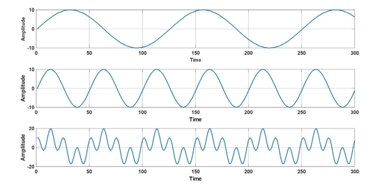
Figure 1: Examples of stationary signals

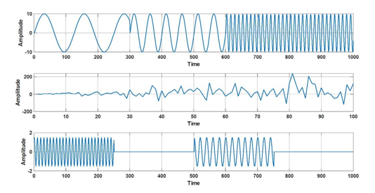
Figure 2: Examples of non-stationary signals

B. Fourier Transform

The Fourier transform (FT) is a mathematical technique widely used to convert a mathematical function or a physical signal from the time domain x(t) to the frequency domain X(ω) to discover the spectrum characteristics of the signal. The conventional equation of the FT is given by [2]:

where x(t) refers to the time domain signal, X indicates the FT of an integrable function, ω expresses the value of the angular frequency, and j represents the imaginary number. FT decomposes a complex waveform into a sequence of simpler basic waves (more precisely, a weighted sum of sines and cosines). FT works best for stationary signals where the statistical characteristics of a signal (e.g., the mean value and the auto-correlation function) do not change with time. FT provides signal information that describes the signal characteristics in the frequency domain. However, it does not tell when these frequencies occur in time [10].

C. Short Time Fourier Transform

STFT is a method developed to add time information to the FT. STFT is designed to overcome the poor time resolution of FT. STFT computes the FFT of short-duration segments of a long signal. This is achieved by multiplying the longer signal x(n) by a small sliding window w(n). The equation of STFT is given by [5]:

STFT can be applied to non-stationary signals by assuming that each small portion of the non-stationary signal is station- ary. The weakness of the STFT is that it employs windows with a fixed length which means fixed resolution in time and frequency for the entire signal.

D.Welch’s Method

The Welch algorithm is a method to calculate the power spectral density (PSD). Unlike the FFT where the PSD is computed over the whole duration of the signal, in the Welch algorithm, the signal is divided into windows of the same size and the FFT is calculated for each window. The size of the window impacts the clarity of the results by cutting frequencies with a duration bigger than the window. Window- ing is defined by taking a sample of a larger data set and tapering the signal at the edges of each period. This makes the signal smoother and avoids the quick transitions which can misrepresent the frequency spectrum representation [11]. Windows which are built-in in MATLAB such as Hamming rectwin, and Blackman, which influence the result differently. Figure 3 shows different windows. Each window overlaps the neighboring windows by a certain factor, which can be as much as 50% of the entire window size. Overlapping allows for decreasing the information lost because of the tapering. Consider a discrete time signal x composed of N samples such that:

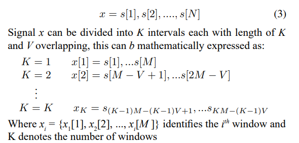
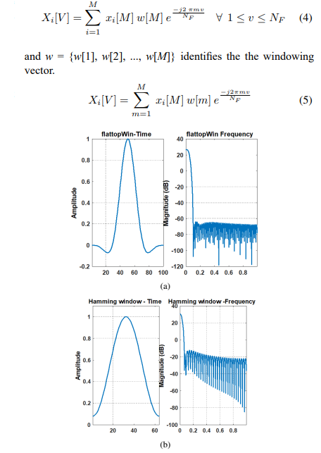
Figure 3: Examples of built-in MATLAB windows (a) rectwin window (b) Hamming window

Wavelet FT utilizes the basic functions (sequence of sine and cosine functions). These functions have frequency contents which do not vary with time, and there which are not well suited for non-stationary signals. Non-stationary signals appear in many applications such as medical applications [13]. The ability to measure non-stationary signals has a broad scope of utility. The limitations of using a fixed size window are shown in Figure 4.

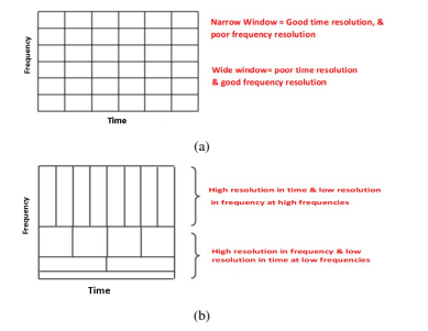
Figure 4: Windowing in frequency and time domains (a) fixedsize windowing size (b) Adaptive windowing

Unlike STFT, where the window size is fixed, the wavelet transform promotes windows with varying sizes to analyze various bandwidth segments within a signal. Mathematically the wavelet transform of a signal f(t) is given by [13]:

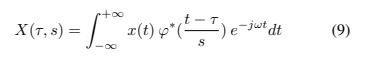
Wavelet transform offers the proper time resolution for the higher frequency parts of the signal and the proper frequency resolution for lower frequency parts. Figure 5 shows how a wavelet can be scaled and shifted to be used for different resolutions.

Figure 5: Shifted and scaled wavelet

Introduction

The time-frequency signal analyses seek to study the main features of the signals by performing time-frequency trans- formations. Stationary signals do not change their statistical properties over time. On the other hand, non-stationary signals vary randomly and change their properties over time [1]. Typically, most signals applied in communication systems, such as audio and video signals, are non-stationary signals. Several traditional and modern methods are commonly used to process stationary and non-stationary signals in which signals are transformed from time-domain to frequency-domain and vice versa. The main concept of time-frequency analysis is to develop a joint function, which can characterize the signals attributes in a time-frequency domain. Time-frequency transforms convert a one-dimensional function of time x(t) into a two-dimensional function of time and frequency. Fourier Transform (FT) was introduced by Joseph Fourier [2]. FT is the most widely used method for spectrum analyses. For instance, most of the available spectrum analyzers are FT based. FT can be described as a harmonic analyzing method that decomposes the analyzed wave into a superposition of sinusoids (more specifically, a weighted sum of sines and cosines). While FT gives an actual representation of station-ary signals in the frequency domain, FT provides spectrum analyses without providing time information. For example, FT analyses can recognize the spectrum features but are not able to localize when these features occur in time. Also, FT is an averaging-based method which assumes the analyzed signals are periodic [2]. This makes FT unsuitable for non-stationary signals [3]. FFT is a version of FT developed by Cooly and Tukey (1965) [7]. To analyze a signal composed of n samples, FFT reduces the required number of computations used by FT from N 2 to N • log2N [3]. Short-Time Fourier Transform (STFT) was introduced by Gabor to overcome the drawbacks of FFT [4]. STFT considers only short-duration slides of a longer signal and calculates its Fourier transform [5]. STFT is achieved by multiplying a longer time function x[n] by a window function w[n], which has a smaller duration [6]. Although STFT can provide concurrent time and frequency localization, it still has a fixed resolution limited by using windows with fixed lengths for low and high frequencies [7]. Furthermore, STFT uses sines and cosines waveforms to compose signals. These waveforms are distributed over the whole signal’s time, and subsequently have infinite energy. Unlike STFT, wavelet techniques use wavelets, which have a short duration, finite energy, and variable window sizes for different signal frequencies [8].

Tools of Analyses

A. fft Function

fft() is a MATLAB function that can calculate the DFT of any sequence or signal. Furthermore, fft() is described as an algorithm that transfers a sequence or signal from the original domain to the frequency domain.

B. stft function

i=1 stft() is a MATLAB function that computes the STFT of the time- domain input signal. The function takes the time- domain signals and buffers them to the window length and overlap length given by the user. Then, it multiplies the samples by the window and computes the FFT of the buffered windows.

C. pwelch function

The Welch method is a widely used method to estimate PSD from EEG. Welch method utilizes a moving window approach where the FFT is calculated in each window and the PSD is then computed as an average of FFTs over all windows. This is performed by employing the pwelch() command in MATLAB. PSD estimation using Welch’s method depends on the window length, the percentage of window overlap, and the number of FFT points. Although it is possible to apply different windowing functions, the Hamming window is the most commonly used because it has good frequency resolution and reduced spectral leakage.

D. Signal Analyzer

Toolbox The Signal Analyzer MATLAB toolbox represents an in- teractive interface that can visualize, process, characterize, analyze, and compare signals in both time and frequency domains. Signal Analyzer MATLAB toolbox provides easy access to the signals in the MATLAB workspace. Through this access, it is possible to process and compare multiple waveforms.

E. Wavelet Analyzer Toolbox

The Wavelet MATLAB Toolbox is an interactive tool that provides functions and tools to analyze, process, and add and extract features from stationary and non-stationary signals. Wavelet Toolbox enables filter, denoise, and multi-scale analysis of images. 

Simulation Results

A. FT Analysis

For analysis purposes, we utilize two signals. The first signal is composed of three sinusoidal signals of frequencies 16, 40, and 80 Hz concatenated to form a non-stationary signal shown in Figure 6. The second signal is generated using the same three sinusoidal signals with the same frequencies. These signals are summed to form a stationary signal shown in Figure 7

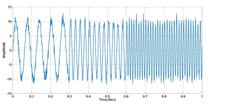
Figure 6: Non-stationary signal composed of , 16 ,40 and 80 Hz

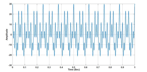
Figure 7: Stationary signal composed of , 16 ,40 and 80 Hz

Figures 8 (a) and 8 (b) show a stationary signal and its FT, respectively. Note that, the FT indicates three components at 16, 40, and 80 Hz, which is explained in the time represen- tation of the signal in the time domain shown in Figure 8 (a). Applying FT analysis on stationary signals gives accurate results.

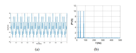
Figure 8: FT analysis of stationary signal (a) Non-Stationary signal (b) PSD of stationary signal using FFT

On the other hand, Figure 9 (a,b,c,d) explains the FT of a non- stationary signal and its flipped version. Although the signal structure is changed in the time domain, the FT displays the frequency components of the flipped signal in the same order as it is in the unflipped version of the signal, which clarifies that the FT is not the best solution for spectrum analysis of the non- stationary signals.

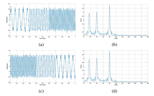
Figure 9: FT analysis of non-stationary signal (a) Non-stationary signal (b) FT of non-stationary signal (b) flipped version of the signal (d) FT of flipped non-stationary signal

B. Periodogram Method

The periodogram is a nonparametric estimate of the PSD of a signal. PSD estimate is obtained by splitting the time signal into successive segments, forming the periodogram for each segment, and averaging. Periodograms are formed from non-overlapping successive data segments. Welch’s method represents an improvement of the Periodogram method. In Welch’s method, the data segments might overlap. Figure 10 compares the power spectrum analyses using Welch’s and the Periodogram methods.

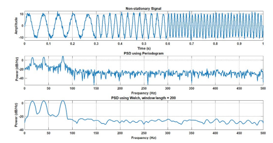
Figure 10: Analyses of non-stationary signal composed of , 16,40 and 80 Hz using Periodogram method

C. Welch Function

Figure 11 shows the power spectrum analysis of a stationary signal using Welch’s method of windows of lengths of 200 and 100 respectively. The figure shows peaks at the frequencies 16,40, and 80 Hz. The difference between using windows of different lengths appears in the resolution.

Figure 11: Analyses of stationary signal composed of , 16 ,40 and 80 Hz using Welch’s method

Figures 12 and 13 display the power spectrum analyses of a non- stationary signal and its flipped version respectively. Notably, Welch’s method shows the power peaks of the non- stationary signal, and its flipped version in the same order, which does not match the time representation of the flipped version of the non-stationary signal. This verifies that Welch’s method works best for stationary signals, while it does not represent the best solution in the case of non-stationary signals.

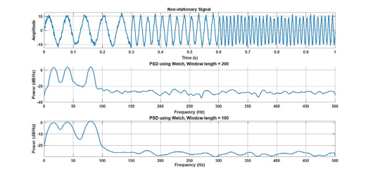
Figure 12: Analyses of non-stationary signal composed of , 16 ,40 and 80 Hz using Welch’s method

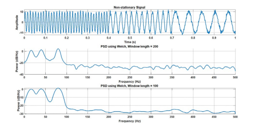
Figure 13: Analyses of flipped non- stationary signal composed of , 16 ,40 and 80 Hz using Welch’s method

D. STFT

Figures 14 (a) and 14 (b) display the STFT analyses of a stationary signal using the rectwin and hamming windows of a length of 100. Figure 14 (b) provides a higher resolution than Figure 14 (a). Note that because we are analyzing a stationary signal with the same pattern repeated, the three signal frequencies appear as three continuous lines.

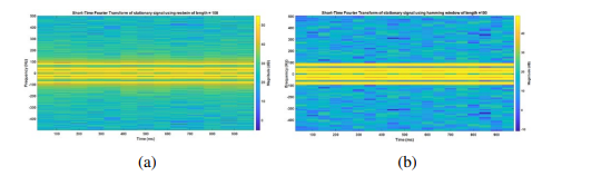
Figure 15: STFT analyses of non-stationary signal (a) using rectwin window (b) using hamming window

Figures 16 (a) and 16 (b) display the spectrum analyses of the flipped version of the stationary signal. These figures clarify that the spectrum analyses of non-stationary signals can be handled using the STFT.

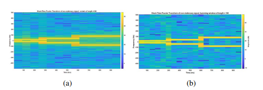
Figure 16: STFT analysis of flipped stationary signal (a) using rectwin window (b) using hamming window

  E. Wavelet

Figures 17 (a) , 17 (b), and 16 (c) display the wavelet-based draw of stationary signal, non-stationary signal, and flipped version of the non-stationary signal respectively.

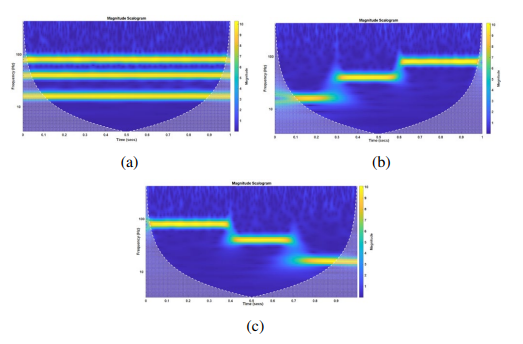
Figure 17: STFT analyses of flipped non-stationary signal (a) using rectwin window (b) using hamming window

F. Wavelet Denoising

Because non-stationary signals are composed of numer- ous physically meaningful elements spread over the entire spectrum of the signal, it is always desirable to analyze these elements separately in many applications using multi- resolution analyses.

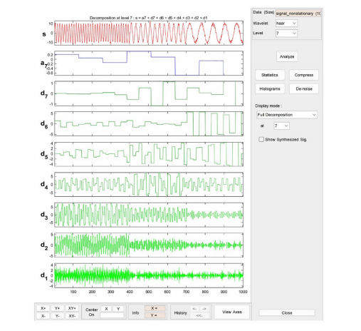
Figure 18: Non-stationary signal decomposition using MATLAB

Multi-resolution analyses refer to splitting up a signal into elements, which construct the original signal precisely when summed back together. The signal elements typically describe the variability of the signal into physically meaningful and interpret-able components. As seen in Figures 14, 15, 16, and 17, STFT and Wavelet analyses give very good results for stationary and non-stationary signals. Besides, wavelet decomposition represents a powerful tool for multi-resolution analysis of non- stationary signals. For example, applying frequency wavelet-based multi-resolution analyses on non- stationary signals can play a significant role in filtering out the noise based on the noise frequencies. This process is referred to as wavelet-based de- noising. Wavelet-based de- noising is very important in the case of non-stationary signals where using power thresholding is not efficient due to the nature of the non-stationary signals, which are composed of variable amplitude components. Figure 18 shows how to use the MATLAB wavelet analyzer in analyzing the components of a non-stationary signal.

 G. Measuring the Occupied Bandwidth of Stationary and Non- Stationary Signals

The occupied bandwidth of a signal is defined by the frequency range that contains a certain percentage of the total spectral power of the signal. There are different criteria used to calculate the occupied bandwidth of any signal. One criterion is by calculating the distance between two zeros of the power spectral density.

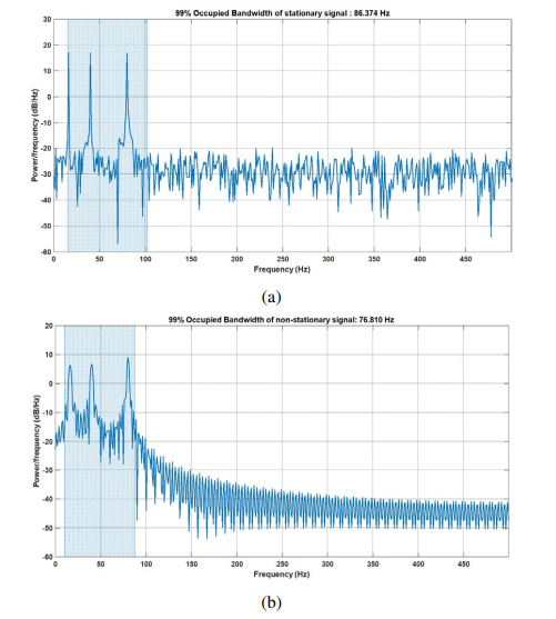
Figure 19: The occupied bandwidth of (a) stationary signal (b) non-stationary signal

The other criterion is figuring out the minimum positive frequency value in which the power spectral is equal to zero. Another criterion is by calculating the frequency band that corresponds to 95% (or 90%, or 99 %, and so on) of the signal power. The criterion adopted by the Federal Communications Commission (FCC) and also implemented by MATLAB de- clares that the occupied bandwidth is the band that utilizes half

of the signal power between the upper and lower band limit. It is also named 99 % bandwidth. Figure 19 (a) shows the occupied bandwidth of a stationary signal composed of the summation of three sinusoidal signals of frequencies 16,40, and 80 Hz. Figure 19 (b) gives the occupied bandwidth of a non-stationary signal composed of three sinusoidal signals of the same frequencies combined.

Conclusion

Time-frequency analyses of non-stationary signals in a noisy atmosphere is a demanding research topic in many fields. They usually require concurrent signal analyses in the time and frequency domains. That is because non-stationary signals are composed of multiple frequencies and irregularly varying am- plitudes in time. Non-stationary signals do not have repeated patterns that might be easily distinguished and simulated. In this paper, and using MATLAB, we comprehensively study different methodological approaches and mathematical tools for non-stationary analyses and compare the outcomes when implemented to stationary signals. Although, our results show that both STFT and wavelet transforms can display a con- junction relationship of stationary and non-stationary signals in frequency and time domains simultaneously, the features of the wavelet MATLAB toolbox appear as very powerful tools, in terms of decomposing non-stationary signals into physically meaningful components. Decomposing non-stationary signals is very useful in terms of denoising where thresholding-based filtering methods are hard to implement.

References

1. Frei, M. G., & Osorio, I. (2007). Intrinsic time-scale decomposition: time–frequency–energy analysis and real- time filtering of non-stationary signals. Proceedings of the Royal Society A: Mathematical, Physical and Engineering Sciences, 463(2078), 321-342.
2. Fourier, J. B. J. (1888). Théorie analytique de la chaleur(Vol. 1). Gauthier-Villars.
3. Heideman, M., Johnson, D., & Burrus, C. (1984). Gauss and the history of the fast Fourier transform. IEEE Assp Magazine, 1(4), 14-21.
4. Gabor, D. (1946). Theory of communication. Part 3: Frequency compression and expansion. Journal of the Institution of Electrical Engineers-Part III: Radio and Communication Engineering, 93(26), 445-457.
5. Cooley, J. W., & Tukey, J. W. (1965). An algorithm for the machine calculation of complex Fourier series. Mathematics of computation, 19(90), 297-301.
6. Rahman, M. (2011). Applications of Fourier transforms to generalized functions. WIT press.
7. Czerwinski, R. N., & Jones, D. L. (1997). Adaptive short- time Fourier analysis. IEEE Signal Processing Letters, 4(2), 42-45.
8. Y. Nievergelt. (1999). Wavelets made easy. Springer, 174.
9. Antoni, J. (2006). The spectral kurtosis: a useful tool for characterising non-stationary signals. Mechanical systems and signal processing, 20(2), 282-307.
10. Bendat, J. S., & Piersol, A. G. (2011). Random data: analysis and measurement procedures. John Wiley & Sons.
11. Marple, L. (1980). A new autoregressive spectrum analysis algorithm. IEEE Transactions on Acoustics, Speech, and Signal Processing, 28(4), 441-454.
12. Parhi, K. K., & Ayinala, M. (2013). Low-complexity Welch power spectral density computation. IEEE Transactions on Circuits and Systems I: Regular Papers, 61(1), 172-182.
13. Mallat, S. (1999). A wavelet tour of signal processing. Academic Press.