The Story of the Electric Charge ‘e’ of the Electron

Introduction

In the mainstream of Physics, the electric charge e of the electron is considered as a universal constant. Its numerical value has been determined by the oil-drop experiment of Millikan: e = 1.602 x 10-19 C. In his Nobel lecture (1923) he said this value mainly depended on the physical conditions of the experiment: the velocity of the oil-drop and the electric field used in the experiment. So, if these physical conditions change, the measured value of e would change accordingly. In other words, the constancy of e is a mere assumption or postulate for the convenience of the research of physics.

That’s why in the contemporary physical literature we can find various statements by prominent physicists who expressed the variability of the electric charge of the electron in different ways:

• Bekenstein " Thus, every particle charge can be expressed in

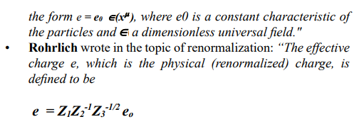
where Zi are renormalization constants .”

• David Griffiths wrote in the textbook Introduction to Elementary Particles: “The effective charge of any particle is somewhat reduced:

q_eff = q / €”

where € is the relative permittivity of the particle. Interestingly, Figure13.1 in the textbook Nuclear and Particle Physics by W.S.C. Williams shows that the electric charge | e | of the electron changes with the distance r.

This is Figure 1 of the electron in the textbook “Nuclear and Particle Physics” by W.S.C. Williams. This figure explains the phenomenon of vacuum polarization and at the same time suggests that the variability of the electric charge e of the electron is physically plausible.

It is the unique figure that supports the idea that the magnitude |e| of the electric charge of the electron is an effective one: it changes with the probing distance r. This means that e is actually a multi-valued factor, not a single-valued constant.

Therefore if we consider the electron as an extended particle, composing of a negatively charged core (-q0), surrounded by a cloud of tiny electric dipoles (-q, +q) as shown in the above figure, we can prove that its effective electric charge e depends on its velocity , external applied field, its permittivity €, its permeability µ and also on the stage of emission & absorption of photons of the electron [1].

First, let us define the meaning of the following letters that are used in this article:

- (-q, +q): electric charges at two ends of the electric dipoles which form the extended electron,

- q or Q or e: effective electric charge of the extended electron,

- q0: constant electric charge of the core of the electron: q0 = e0 = 1.602 x 10^-19 C

Three New Equations of the Effective Electric Charge

In this article, I introduce three new equations that I created to describe the variability of the effective electric charge of the electron. Since the calculations are lengthy, only the results (i.e., the equations) are given here; the proofs of calculations are referred to the references at the end of the article

A Heuristic Mathematical Expression of the Electric Charge:

where = (1-v² /c²)-^1/2 is the Lorentz factor, N ≥ 0 is the real number representing the external applied field. This equation is the result of a heuristic argument, it is not derived from the calculation on the extended electron [2]. The equation shows that the effective electric charge of the electron is a function of its velocity v and the applied field represented by the positive real number: N ≥ 0.

Figure 2: q / q 0 = (1 – v2 / c2) N/2

From the graph we notice that the higher the field (larger N) and / or the higher the velocity, the more the electric charge approaches zero.

In low fields (N = 0.5, 1.0) the electric charge does not become zero even when v tends to c. In higher fields (N = 10, 20, 50) the electric charge of the electron becomes zero when v /c ≈ 0.8. This means that the electron can become a free electron (has no electric charge at all) at the velocity less than c (e.g., v ≈ 0.8 c) provided that the applied field must be high (N = 20 to 50).

The equation q / q0 = (1 – v² / c²) ^{N/ 2} shown in Figure 2 illustrates the effect of the applied field N on the effective charge q, especially for very high N. Because (1 – v² / c²) < 1 for any value of the velocity v, the factor (1 – v² / c²)^N/2 tends to zero when N is very high, and hence q tends to zero. This equation is the unique equation in physics that depicts the change of the electric charge of the electron with the applied field (just because mainstream physics assumes the electric charge of the electron is a constant!).

Equation of the Effective Electric Charge in Electric Field:

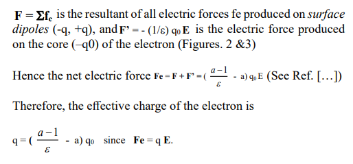
where € is the relative permittivity of the electron, ‘a’ is the dimensionless form factor derived from the structure of the extended electron in electric field [3].

Method of calculation: since the extended electron has two charged components: the surrounding cloud of electric dipoles (-q, +q) and the core (-q0), when it is subject to the applied electric field E, two different forces are produced on these two components:

Equation of the Effective Electric Charge in Magnetic Field

By associating these three equations we will discuss two subjects that are closely related to the effective electric charge of the extended electron:

1 / Renormalizing the Lorentz’ s force equation to expand it into the relativistic regime.

2 / The conversion Particle ↔ Anti-Particle of Dirac & Majorana

Renormalizing the Lorentz’ s Force Equation

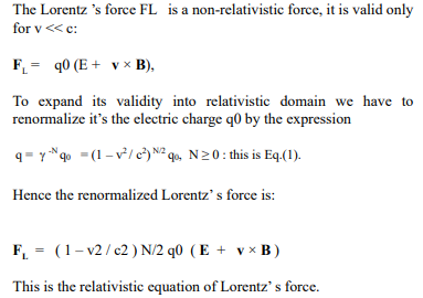
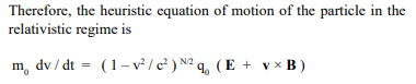
That is, Classical Newtonian force = Relativistic Lorentzian force [5]. The immediate consequence of renormalizing Lorentz ' s force is that the electric force

• Fe and the magnetic force Fm tend to zero as v → c for anyvalue of the applied field N:

• Fe = (1 – v2 / c2) N/2 q 0 E: Fe decreases with v (from v = 0)and tends to zero as v → c

.• Fm = (1 – v2 / c2 ) N/2 q 0 v × B : Fm increases with v (from v = 0) reaches its maximum at v = c (N + 1)-1/2 , then decreases and tends to zero as v → c.

Notes:

• The maximum point of Fm is an intriguing point: there are two different values of velocities V1 and V2 (on either sides of the maximum point) that give the same value of Fm.

• I would like to call on the readers who are proficient in computer graphics: please delineate the graphs of Fe and Fm with N = 0, 1, 2…50 …100… as functions of the velocity v to see how they tend to zero as v c. We also notice that when we renormalize the Lorentz ’s force, both Fe and Fm move down and lie below the familiar forces Fe and Fm in non-relativistic regime (Fe = q0 E and Fm = q0 v × B).

Discussion: In classical physics, physicists noticed that Newtonian force FN is not equal to the Lorentzian force FL: it is lower than the Lorentzian FL. They tried to bring them to equality by increasing FN (by renormalizing the mass m0 in FN) by the factor

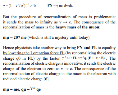
That is: the mass of the muon is equal to the mass of the electron, but its electric charge is time smaller than that of the electron. The idea that all muons which are created in different conditions (in the labs or in the upper atmosphere …) have the same charge and the same lifetime (2.2 µs) is incorrect. Thereby, the concept of time dilation, which relies on the idea that all muons have the same lifetime (2.2 µs), is wrong and superfluous for physics.

Conclusion: muon is not a heavy electron; its average lifetime tau is not always equal to 2.2 µs but changing with velocity and the external field where it is created. These findings lead to the ascertainment that the concept of time dilation is wrong and redundant [7].

The Conversion Particle Anti-Particle of Dirac & Majorana

Determination of the net Electric Force Fe Produced on the Extended Electron

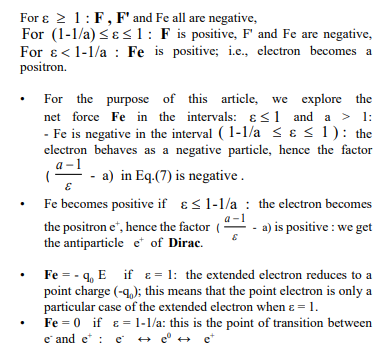
When the extended electron is subject to an external electric field E, the net electric force Fe is produced on it. The calculations on the extended model of the electron show that Fe is the resultant of two opposite forces F and F’, i.e., Fe = F + F’ , where F is the

 

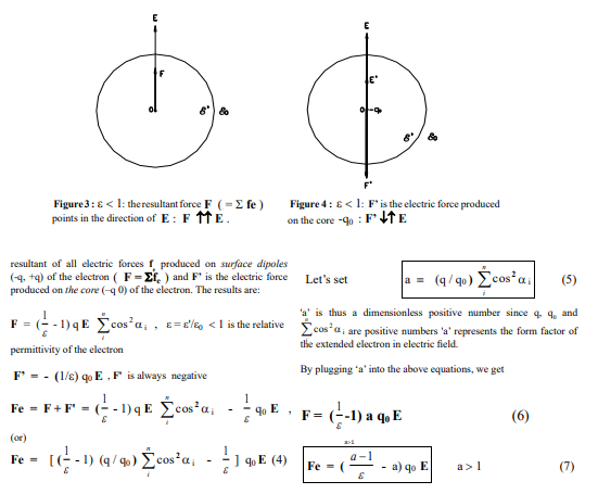
            Figure 5: Shows F, F' and Fe as functions of ε.

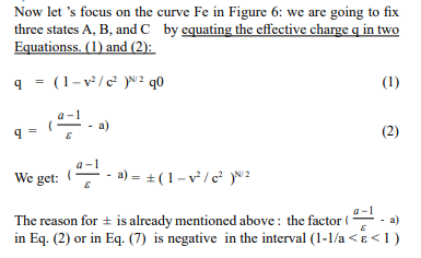
The ephemeral state e0 appears to be the Majorana particle, which is its own antiparticle. At this state, the particle (e -) coincides with its antiparticle (e +). This is the state of the electron at the point B: ε = 1 - 1/a , Q = 0 , v = c as shown in Figure 6 of the next section

Therefore, the variability of the permittivity ε of the extended electron under the action of the applying field changes its effective electric charge Q and hence the direction of Fe. Owing to the direction of Fe with respect to the field E, we recognize the particle being an electron or a positron. The consequence is that the electron can undergo different states from e- to e+ via eo . e0. In short, antiparticle originates from its particle and vice-versa, due to the variability of its permittivity ε which causes the change in its effective charge.

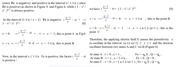
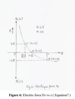
Note: Let 's note that Dirac predicted the existence of the antiparticle e+ from his relativistic wave equation, but he did not elaborate how e+ was created physically; i.e., he did not explain what was the mechanism of its generation. And yet he was awarded the Nobel prize in 1933 after e+ was discovered. As for the theoretical particle Majorana: it is the conversion point of particle and antiparticle; or in other words: it is the transition point where the particle coincides with its own antiparticle. This is the point B in Figure 6, where : ε = 1 - 1/a , Q = 0 , v = c ; meanwhile two points A and C are turning points , where v = 0 and the acceleration changes its signs

Fixing Three Points A, B and C on the Curve Fe (Equation 7)

 

Magnetic Force Fm and Three Points A, B, and C

Using similar method of determining the force and fixing three points A, B and C, we will determine the magnetic force Fm which is produced on the extended electron by the applied magnetic field B and fix three points A, B and C on the curve Fm.

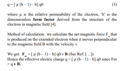
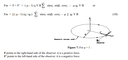
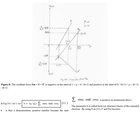
Now, let ' s investigate the magnetic force Fm which is produced on the extended electron when it moves normally to the external magnetic field B with velocity V. The results of calculations For μ > : F points to the right-hand side of the observer as shown in Figure 7: it is considered as a positive force; and hence the sum n showed that the resultant force Fm composes of two opposite forces F and F' as shown in Figure 7.

F is the resultant of all magnetic forces fm produced on surface

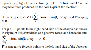
The resultant magnetic force is Fm = F + F’:

Search for the Point B

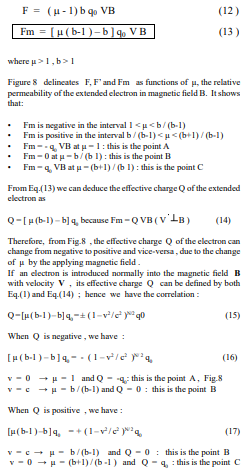
On two Figs. 6 and 8 three points A, B and C represent three particular situations of the electron: while two points A and C represent the turning points of the electron (where v = 0), the point B represents the situation (or state ) where electron is converted into positron and vice versa :

We think that the point B physically exists, we can experimentally determine the point B , at which electron is converted into positron and vice versa .

We can perform experiments to demonstrate the existence of the point B by changing É? or µ by using laser to impact electrons before injecting them through the applied electric or magnetic field. When É? or µ reaches the point B: É? = 1- 1/a, or µ = b/ (b-1), electron turns into positron: it reverses its direction of motion in the electric field E, or it deflects to opposite direction in the magnetic field B.

This is the conversion: particle ↔ antiparticle. This conversion occurs at a specific point, called point B or Dirac-Majorana point.

In contemporary physics there are two similar phenomena: The Curie point (Curie temperature) at which a magnetic material is transformed from non-magnetic into magnetic: paramagnetic ↔ ferromagnetic. Also, in the superconductivity, there exists a very low temperature near zero K0 that changes a normal conductor into a superconductor.

All these phenomena link to the change in the electric charge (or the magnetic moment) of a single electron which undergoes a change in its permittivity É? or its permeability µ.

I would like to call on researchers around the world to carry out this experiment to spot the point B of the electron in E and B.

If the experiment succeeded, it would explain the mechanism of the conversion of particle ↔ antiparticle which Dirac and Majorana had predicted.

Conclusion

This is a short story of the effective electric charge ‘e’ of the extended electron. It is a part of more important features of the electron: the spin & radiation of the electron, the emission & absorption of photons. These subjects are presented in my book: “A new theory of the extended electron” which will be published this year (2026) by SCIRP, attempting to open a new road to the new physics.

References

1. Nguyen, H. V. (2026). “Emission & Absorption of Photons of the Extended Electron in Electric Field”. Journal of Electrical & Electronics Engineering. ISSN 2834-4928. Vol.5 Issue 2.
2. Nguyen, H. V. (2021). A Fundamental Problem in Physics(Mass vs Electric Charge)”. vixra : 2109-0010.
3. Nguyen, H. V. (2013). “Extended Electron in Constant Electric Field”. vixra :1306-0235.
4. Nguyen, H. V. (2013). “Extended Electron in Constant Magnetic Field”. vixra: 1309-0105.
5. Nguyen, H. V. (2021). “A Theory of the Extended Electron”. vixra : 2105-0043.