The Physical Principles of Non-Shared Coordinate System

Theoretical Background of the NSCS Physics Principles

Physics, as an experimental science, relies on advancements in measurement techniques for its development. The introduction of coordinate systems marked the transition of physics from qualitative to quantitative analysis. In practical applications, coordinate systems are objectively divided into observational coordinate systems (the coordinate system held by the observer) and background coordinate systems (constructed by the time axis and space axis, representing the spacetime background of the observed physical phenomena). During the Galilean-Newtonian era, it was unnecessary to distinguish whether the coordinate system used to read the measured space-time data was an observational coordinate system or a background coordinate system. However, as physics has entered the NSCS stage, although the observer remains the subject performing measurements, there are now two sets of measurement tools, or coordinate systems, to choose from. Which coordinate system should be chosen as the reading data coordinate system has become an unavoidable top-priority topic. Relativity chose the traditional approach: the observer's own coordinate system is used to take readings [1] (P20) [6] (P60). This leads to the well-known conclusion: the spatial length along the direction of motion and gravity contracts at the same ratio, whereas the length perpendicular to this direction remains unchanged. While the conclusions of time dilation and the contraction of lengths in the direction of motion have been supported by experiments, the conclusion that 'lengths in the perpendicular direction remain unchanged'has thus far never been verified experimentally. It is precisely this unverified conclusion led to the 'three-dimensional difficulty' in special relativity: physical laws, such as Coulomb's law, that involve three-dimensional spatial coordinates simultaneously in mathematical expressions are not covariant, similar to Newton's universal law of gravitation. General relativity, developed specifically to avoid the non-covariance of Newtonian gravity, but also introduces additional difficulties. For example, structural contradictions of such as the non-conservation of energy and angular momentum in a gravitational field [2] (P84), are irreconcilable with quantum theory and are unable to solve physics puzzles such as quasars, dark energy, and dark matter.

Want to calm down the many disputes in quantum mechanics (as another pillar of 20th-century physics), such as the peculiar behavior of quanta and the explanation of wave-particle duality, etc., are also closely related to the choice of the reading coordinate system. The difficulties faced by each own of the two incompatible theoretical systems unexpectedly point to the same origin, which is certainly not mere coincidence.

Fundamental Principles of NSCS Physics

Original Topic: Who is Qualified to Serve as The Coordinate System for Reading Data

In classical physics, an observational coordinate system is established on the basis of the reference object, with all observed objects situated within this coordinate system. Therefore, this coordinate system also serves as the spacetime background coordinate system for those observed objects. The position data of all the objects (which can all be considered point masses) at any given moment all readings are taken via this coordinate system. Therefore, the time and space standards of this coordinate system are the unique standards for measuring time and space across the entire examined area. The clocks and rulers that move with the observed particle have no opportunity to be used. This is the underlying reason why no one cares about whether moving clocks slow down or moving rulers shorten during the SCS stage, and it also forms the subconscious psychological basis for the collective mentality of 'using the observer's coordinate system for readings'.

When the observed object can no longer be treated as a mass point, but rather requires observation of the motion of mass points contained within it, the background coordinate system that originally served dual purposes as the observation coordinate system during the SCS stage can no longer share the same coordinate system with an external observer. At this point, it is necessary to select a coordinate system for the observer as the measurement tool. Throughout human history, both of these options have been used to describe the movements of the major planets in our solar system: Observers on Earth use their geocentric coordinate system for observations, resulting in geocentric theory; measurements made using the heliocentric coordinate system are referred to as heliocentric theory. From a geometric perspective, both measurements are valid, but from a physical standpoint, only heliocentrism can provide a reasonable explanation for the behavior of major planets. A physical explanation can be made because the heliocentric coordinate system serves as the background coordinate system for the orbits of planets within the solar system. Heliocentrism could or inevitably replaced geocentrism not because it provided a more concise and mathematically elegant description, but because it better aligns with physical logic. Behind this logic hidden one Nature Original Commandment—only the background coordinate system is qualified to serve as the reading data coordinate system. Heliocentrism and numerous everyday experiences indicate that background systems in physics research are naturally formed and cannot be arbitrarily designated by humans, unlike observation systems. Forcing the designation of a background coordinate system artificially is not only meaningless but also leads to paradoxes. The SCS stage measurements did not violate this Original Precepts either because, at that time, the coordinate system had dual roles of observation system and background system, and the measurement actually used the background coordinate system function, although people mistakenly thought it was the observational coordinate system.

The Measurement Principles of One Person Measuring Two Systems

Set there are three large ships on the calm water surface: Ship A is stationary on the water surface, whereas ship B and ship C are moving at constant speeds of 0.6 and 0.8 times the speed of light, respectively. When making mechanical experiments in each ship separately, Galileo discovered the following: if observers on each ship observe only experiments conducted on their own ships (abbreviated as oneself measure oneself), the same experiment exhibited identical results on each ship. Since large ships at rest and moving at constant speed both belong to inertial frames, this phenomenon is also summarized as 'all inertial frames are equal'. Later, it was further reinforced by the principle of special relativity, people's focus shifted towards whether a reference frame is an inertial frame, whereas the core concern of choosing the reading coordinate system was overshadowed.

When Einstein opened the windows and doors of Galileo's Great Ship, physics arrived at the front door of the NSCS. Without windows or doors obstructing the view, an observer could be someone from another ship. When an observer on ship A measures the motion of particle P inside ship B, should A use its own coordinate system or utilize B's coordinate system? This becomes the first fundamental issue encountered during the NSCS stage. Following the Nature Original Commandment, the A coordinate system is not the spacetime background for P and therefore lacks the qualification to measure P's motion data. Observer A must utilize the B coordinate system to measure P's data. A's measurement of P is achieved through two steps: Coordinate system A is the spacetime background for the motion of ship B, which can be used to read B's motion data and thereby calculate the ratio at which B's coordinate system spacetime contracts relative to A. At the same time, the observer on ship A uses the background coordinate system of P, which is the coordinate system of ship B, to read the data of P's movement in the B coordinate system. By dividing the spacetime coordinate difference read from the B coordinate system by the spacetime contraction coefficient observed by A of the B system, it is what we get the data of P's movement observed by A. This two steps correspond to two the measurements: a direct measurement and an indirect measurement. For the fast or slow of the same clock and the long or short of the same ruler, if two observers Oneself Measure Oneself, will result in identical experimental reports. The observers in the two systems measure each of the same experiment conducted in the coordinate system of the other party, and the obtained experimental reports would be also identical. Only by combining these two measurement methods: Ship A's observer repeat the experiment that P conducted on ship B within A, and measure the data for Experiment P on ship A (A measure A); At the same time, observer A using coordinates system B measure data of P in system B (A measure B ); Comparing the two measurement results allows us only then to identify the similarities and differences of the same experiment in the two systems, or how a standard clock and standard ruler would slow down or shorten in which coordinate system. In simple terms, for measurements of the same experiment on both ship A and ship B, they must all be implemented by one person from Ship A (i.e., A measure A + A measure B) (of course, that can also be implemented by one person from ship B, i.e., B measure B + B measure A). This measurement method is called the one-measure-two. Therefore, the requirements of the One Measure Two were established as the measurement principles for the NSCS stage. It is also the first threshold into the NSCS physics.

Principle of Duality for Reference Frames

In addition to the Measurement Principles, the 1970 cesium atomic clock global circumnavigation experiment provided further constraints. When comparing the fast or slow of an airplane clock and a ground clock according to relativity, you can choose the ground as a reference object. Therefore, whether an airplane flies east or west along the equator, its speed relative to the ground remains the same, and at the same flight altitude, the gravitational potential is also identical. Without even calculations, one can know that the cesium atomic clock flying east and the one flying west either gain or lose time by the same amount relative to the ground clock does. However, the observed values in the actual experiments were as follows: the clock flying east is 59 ns slower than the ground clock, while the clock flying west is 273 ns faster than the ground clock [3] (P61). This precisely negates the practice of arbitrarily designating the ground as the coordinate system for readings. In a natural system composed of an aircraft clock, a ground clock, the Earth, and its atmosphere, the geocenter can only be uniquely selected as the reference to measure the motion rates and gravitational potentials of the three clocks. Only by calculating their respective fast or slow ratios relative to the standard clock and then comparing the fast or slow of the three clocks can the results match the experimental observations. The experiment reveals that when comparing the fast and slow of clocks between observers and the be measured system, there are strict requirements for the pairing conditions of both parties involved: In the physical system under consideration, the speed and gravitational potential of one of the two systems must truly be zero. The coordinate system established on this reference object (its potential and speed are zero) is the background frame of reference for all motion within that system. Facts tell us, in naturally formed physical systems, reference objects that meet these conditions can always be found. Among two reference frames, one must have zero potential and zero speed, which is called the dual condition of the reference frame. A pair of reference frames that meet this condition is called the dual reference frame. One of the significant advantages of reference frame duality is that the roles of the two reference frames can be interchanged: A static Galilean system pairs with a dynamic gravitational field system, and the observer becomes the standard system, whereas the observed one automatically becomes the self-coupled system.

Regardless of who it is, the premise for deriving spacetime transformations is that two reference frames must be dual. Therefore, the spacetime transformation equation can be applied only between the Dual Reference Frames. As previously set, with the water surface as the reference frame, Ship A's speed is zero, so Ships B and A, as well as Ships C and A, form dual relationships, whereas Ships B and C do not meet the Dual Conditions. To compare the fast or slow of the clocks on B and C ships, you must first pair them with ship A separately, calculating that their fast or slow are 0.8 times and 0.6 times that of ship A's clock, respectively. Only then can you determine that for every second B's clock ticks, C's clock is 0.25 seconds slower. If the relative speed of ships B and C, which is 0.2 times the speed of light (considering only the case where they are moving in the same direction), is directly substituted into the time transformation formula, the result obtained is that they are 0.02 s slower than each other every second. This value is not only 12.5 times smaller than that of the previous algorithm but also be a so-called paradox that contradicts each other. Given this, the two reference frames involved in spacetime transformation must meet the objective requirement of the Dual, which is established as the principle of reference frame duality. It is also the second threshold for entering the NSCS physics. Together with the measurement principles, they are known as 'the Two Rules'.

Four-Same Spacetime Theory and Microscopic Mechanisms of Spacetime Contraction

Before introducing a coordinate system, physical quantities are typically composed of numbers that indicate their magnitude and dimensions that represent their physical category:

In equation (2.4-1), only the real number n is associated with the number line. It is represented by the ratio of the length on the number line (the difference between the coordinates of two points) to the arbitrarily chosen unit length of the axis. Moreover, define the ratio of unit physical quantity and unit axis length as the physical metric, so the physical quantities expressed by the number line in the coordinate system are as follows:

In a static Galilean reference frame (abbreviated as the SG system), the physical metric on each spacetime coordinate axis can be arbitrarily defined, but once determined, it becomes a standard metric and cannot be changed at will. Therefore, the SG system is often also referred to as the standard system. When the standard system moves or enters a gravitational field, it becomes a moving and gravitational field frame (abbreviated as the MF system). Each MF system automatically couples a metric that matches its current state based on the basis of its own speed of motion and the gravitational potential at its location. Therefore, the MF system is often also referred to as the auto-coupling system.

When a rigid body moves or enters a gravitational field, the mass of each nucleus and electron within it increases, leading to a greater gravitational force between them. This disrupts the balance between the gravity and Coulomb forces acting on the electrons and the inertial centrifugal force. Under the absolute dominance of Coulomb attraction, the radius of the atom (the space covered by the electron cloud) shrinks, with the centrifugal force increasing until the forces on the electrons reach a new equilibrium. The dimensions of each atom decrease, resulting in the macroscopic dimensions of a rigid body being smaller than those in the SG system. This means that the spatial axis unit length for measuring rigid body linear dimensions (corresponding to the edge length of the spacetime cell grid) contracts proportionally at the same ratio. This is the physical mechanism behind the contraction of space due to motion and gravity. In the new equilibrium state, the atomic dimensions decrease, but the number of energy levels and their geometric distributions remain unchanged. However, each energy level is reduced by the same ratio compared with the corresponding energy level in the old equilibrium. The frequency of photons emitted during a transition between two energy levels under new conditions is, of course, lower than that of photons emitted during the same transition between the same two energy levels under old conditions. This is the microscopic mechanism by which time slows down in motion systems and gravitational fields.

The theoretical calculations to two redshift effects can prove:

• The ratio of change in space and time is the same (abbreviated as space-time same-change).

• The ratio of variation in all space directions is the same (abbreviated as space isotropic).

• The first two change ratios are the same, it has been decided the auto-coupling system's spacetime structure is geometrically similar to the standard system's spacetime structure, i.e., the spacetime structure of the auto-coupling system and the standard system are the same (abbreviated as coupling standard isomorphism).

• Given that motion and gravitational fields unlock the same mechanism that increases the mass of atomic nuclei and their electrons, to trigger the mechanism of space-time contraction, the gravitational potential plays the same role as speed, i.e., the effects of potential and speed are the same (abbreviated as potential-speed same working).

This tells us that there is no need to study separately the transformations of spacetime for the motion system and the gravitational field. Experiments on the transverse Doppler effect of light and gravitational redshift also reveal that motion and gravity can produce not only mechanical-effects within the same system but also spacetime-effects between different systems.

Four-Same Spacetime Interval and Coordinate Transformation Formula

Let reference frame K' move uniformly at speed u in any direction relative to the SG system K, with the corresponding coordinate axes of the two orthogonal coordinate systems established on both frames always remaining parallel (as shown in Figure 1). Now, let us examine the spatial length of the fixed-point P to its origin O' in the moving system K'.

Figure 1: System K' Moves Uniformly at Speed u Relative to Stationary System K

If we assume that the K' frame moves relative to the K frame along the positive X-axis, i.e., u_x 2) becomes = u, u_y = u_z = 0, then equation (2.5-2) becomes

Equation (2.5-3) indicates that even if the K' frame moves along the positive X-axis relative to the K frame, it is impossible for the length of the ruler perpendicular to the direction of motion to remain unchanged.

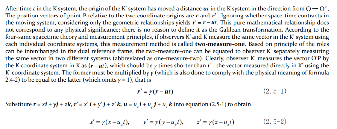
Conversely, observers of the K and K' systems separately measure the K system's vector OP , which is equivalent to an observer in the K system separately measuring the vector OP by one-measure-two, resulting in

Notably, equations (2.5-4) and (2.5-1) are not inverse transformations of each other, as both have quantities measured in the standard system by standard system on their left sides, whereas the right sides involve indirect measurements of quantities in the auto-coupling system by the standard system. The physical meaning of the same letter in the two equations is different, and they are not equivalent. To be equal to quantities measured directly, any quantity measured indirectly must be multiplied by the spacetime contraction factor γ .

To find the value of the spacetime contraction coefficient (or spacetime contraction ratio) γ, for simplicity, let K' move uniformly at speed u along the positive X-axis relative to K, as shown in Figure 2:

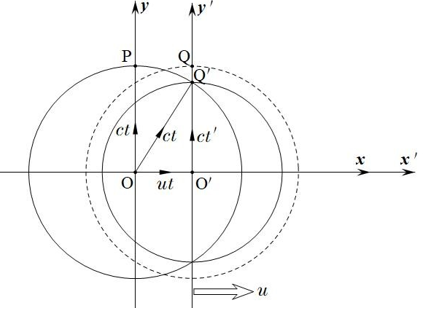
Figure 2: Diagram Showing the Propagation of Light Emitted by A Point Source in the K and K' System

When K' moves so that its origin coincides with the origin of the K system, the point light source at the origin is activated. Two observers from different frames observe the propagation of light within their respective systems (oneself measure oneself). They both see the light emanating from the origin and spreading outwards in spherical waves (projected onto a plane, with wave fronts appearing circular). The radii of the wave fronts ct increase uniformly at the same rate, as shown by the solid large circle and the dashed large circle in Figure 2. Since it is the oneself measure oneself, there is no space and time correlation or constraint between the wave fronts of the two light beams, which are represented by two independent circles.

If let the observer in the K system makes observations of light propagation in two systems (one-measure-two by K), then K is the standard system. He can only make indirect measurements of the propagation data of light in the K' frame by using the K' coordinate system. Since measurements are made via the K' coordinate system, the light wave must still be a circle centered at O'. He measured that K' moves at a speed of u, but it cannot be determined whether the radius of its circle increases faster or slower. Without loss of generality, let its dynamic radius be c't'. From the space-time same-change, we know that the contracted distance divided by the contracted time at the same ratio, i.e., the speed of light c' in K', is inevitably equal to the speed of light c in K. When the same observer measures light waves emitted simultaneously from the same point in both systems, since the light source in the K' system is always on the Y' axis, the wave fronts of the two light waves inevitably intersect on the Y' axis. To ensure that the light in the K system does not exceed the speed of light, the radius of the light wave sphere observed by K in the K' system must be smaller than the radius of the light wave sphere in the K system, as shown by the small solid circle in Figure 2. Thus, the spacetime relationship between the two systems was connected. From the vector triangle OO'Q', we can derive

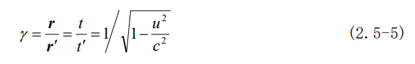
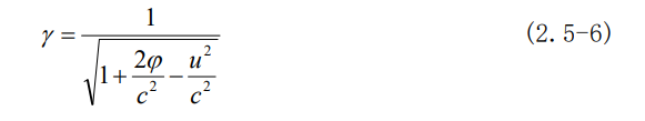
By replacing the uniform motion of K' with uniform acceleration and equating the accelerated motion to a uniform gravitational field, it is easy to determine that the coefficient for spacetime expands or contracts (stretching if φ > 0, shrinking if φ < 0) in a reference frame with gravitational potential φ and velocity u [4] (P104):

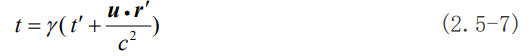
The timing zero point of clock K' when stationary is the same as that of clock K. When K' accelerates from 0 to u, its zero point of time takes different values at different positions in the equivalent gravitational field: ux'/c² [4] (P4-5). These different timing zero points are not automatically be erased when accelerated motion ends. In actual practice, to assume t' = t = 0 when the origins of the two systems overlap, which means that the zero points of all K' system clocks are set to zero artificially. Taking this into account, the time interval transformation formula expressed by equations (2.5-5), which considers only the fast or slow nature of the clocks, becomes a time coordinate transformation formula that takes into account both the fast or slow nature of the clocks and the zero point of timing:

From equations (2.5-4) and (2.5-7), if K uses the K' coordinate system to measure the velocity of a particle in the K' system as v'= dr'/ dt', then the velocity of that particle in the K coordinate system is

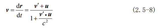
In this vector transformation equation, if v' = c, then it is inevitable that v = c. This indicates that regardless of which star in the binary system which direction to move, the speed of light emitted from any position at speed c always reaches Earth at speed c, without causing the illusion of simultaneous arrival of light from different distances, creating a mirage star, which aligns with actual astronomical observations. This is something that scalar velocity transformation equations cannot achieve.

Combining equations (2.5-4), (2.5-7), and (2.5-6) results in the universal four-same spacetime transformation equation. The spacetime scaling coefficients expressed in equations (2.5-6) have different names for the physical metric from those in equation (2.4-2), but they refer to the same concept. This reveals that the parameters that determine the spacetime metric of the coordinate axes are either the rate (speed) of motion of the reference frame or the gravitational potential at a point in the gravitational field, rather than the two vectors of velocity and gravitational field strength. This also indicates that the contraction of space length, just like the slowing of time, should be independent of the direction of velocity and gravity. Those who believe that space expansion and contraction are related to direction, all of which are due to a failure to distinguish between the mechanical -effects of motion and gravity (in the SCS), and the spacetime-effects of motion and gravity (in the NSCS).

The standard system K uses the K' coordinate system and measures the density of matter in the K' coordinate system as ρ = γ⁴ρ₀ [4] (P241), om the spatial interval transformation formula, when K uses the K' coordinate system to measure the volume of 3 objects in K', it is V = V₀ / γ³(where ρ₀ and V₀ are quantities measured by K in K). Substituting them into the equation relating mass, volume, and density, we obtain the relationship between the MF system mass m and the SG system mass m₀ :

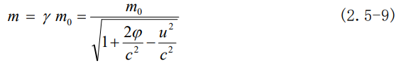
Equations (2.5-9) provide the basis for the increase in the mass of the atomic nuclei and their electrons when a rigid body moves and enters a negative potential gravitational field, as discussed in Section 2.4.

The Physical Mechanisms of Spacetime Bending and the Strategy of 'Using Linear Solve Nonlinear'

The coupling-standard isomorphism indicates, that the high or low gravitational potential at any point in an auto-coupling system does not affect the similarity of spacetime structures with those in a standard system, but it affects the edge lengths of the four-dimensional cubic spacetime cell grid at each point and its neighborhood. When spacetime cell grids of different edge lengths are connected, the spacetime lines formed by connecting edges with the same name are inevitably zigzag lines that do not lie on a straight line. As adjacent points become infinitely close, the zigzag line tends toward a smooth curve. This is the microscopic mechanism of spacetime bending [4]. (P160-162)

To apply classical physics laws in curved spacetime, two conditions must be met simultaneously: 1. The spacetime structure of each point is identical to the spacetime structure at the time when these physical laws were discovered. 2. The same physical law applied at each point automatically has the same mathematical form. In NSCS physics, the spacetime evolution laws of the coupling-standard isomorphism naturally satisfy the first condition. The fulfilment of the second condition requires the use of the principle of relativity, and the principle of reference frame duality unique to NSCS physics. The spacetime points through which the object's motion passes are selected. According to the principle of relativity, observers at these points, observing the same object moving within the same SG system, the physical laws that are followed, inevitably provide the same mathematical form. Each point is paired with that SG system to form the dual reference frame. Since the roles of the dual reference frames can be interchanged, i.e., A observes an experiment for the B system equivalent to B observes the same experiment for the A system, the experimental reports provided by the two observers are inevitably identical. Therefore, the observer at each point of which the object passes, they observe separately the same object moves in the SG system, can be equivalently transformed into the following: the observer of the SG system separately observes the same object moving in the neighborhood of each point.

After the role swap, the SG system observer noted that the physical laws followed by objects within each point neighborhood remained consistent with those observed before the swap, and were described by the same mathematical equations. This naturally satisfies the second condition. The physics of curved spacetime can be handled in the same way as flat spacetime, which is referred to as the strategy of 'using linear solve nonlinear'.

The Application of Classical Physics in the NSCS Stage

With the strategy of using linear solve nonlinear, all issues previously deemed unsolvable by Newtonian mechanics, such as high-speed motion and strong gravitational fields, the gravitational bending of starlight, the 43" per century precession of Mercury's perihelion, radar echo delay, etc., can be solved using Newtonian mechanics just like in the SCS stage, only except for the step of physical quantity transformation.

Classical Physics Remains Applicable at High Speeds and in Strong Gravitational Fields

According to the Lorentz transformation, the rate of clocks and the length of rulers depend on the speed of the reference frame's motion. Time and space are no longer absolute as defined by Newton. Newtonian views of space and time hold only when the speed of motion is negligible compared with the speed of light. Therefore, it is concluded: Newtonian mechanics, even extending to all of classical physics, is an approximate theory for low-speed motion.

For example, the interaction between two stationary objects (both can be considered point masses) follows Newton's law of universal gravitation:

i.e., F∝1/r². If M is located at the origin of the Cartesian coordinate system, the expression for the distance r between m and M is

If M and m move together at the same speed u along the X direction in the stationary coordinate system K, according to the Lorentz transformation, their masses and distances in the moving coordinate system K' are respectively

Although observers in the moving frame of reference (oneself measures oneself) find that the interaction between two objects still satisfies Newton's universal formula of gravitation

i.e., F∝1/r' ². but substituting (3.1-3) into (3.1-4), which means that, from the perspective of the stationary frame, the interaction between the two moving objects is

i.e., F " is not inversely proportional to r². This indicates that the law of universal gravitation of what the stationary system observes in the moving frame can only hold true when u << c.

However, if we use the four-same spacetime transformation equations given by formulas (2.5-9) and (2.5-5), substituting

into equation (3.1-4), we obtain

γ is only a constant related to the speed u, so from the perspective of the stationary system K, regardless of how fast M and m move, their gravitational force satisfies F"∝1/r². Furthermore, on the basis of the principle of potential-speed same working, substituting the Lorentz spacetime contraction factor with the (2.5-6) equation that includes gravitational potential φ, equations (3.1-6) and (3.1-7) still hold true. This is enough to demonstrate, regardless of how strong an external gravitational field may be, as long as the gravitational potential at any point within it has a definite value, the gravitational force between two masses M and m remains consistent with Newton's universal law of gravitation at any point and its neighborhood within this gravitational field serving as the background spacetime, even if both masses are moving at high speeds.

Now let us look at an example from electrodynamics. By substituting the Lorentz transformation equations with the four-same spacetime transformation equations, the component relationships of the electric field intensity E and magnetic induction intensity B between the dual reference frames K and K' as observed by an observer in frame K are obtained [4](P345) as follows:

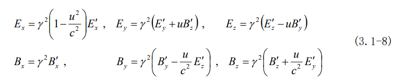
Here, γ represents equation (2.5-6), which includes the gravitational potential φ, indicating that equation (3.1-8) is also applicable in a gravitational field background system.

The first three and last three equations of (3.1-8) are expressed in vector form as follows:

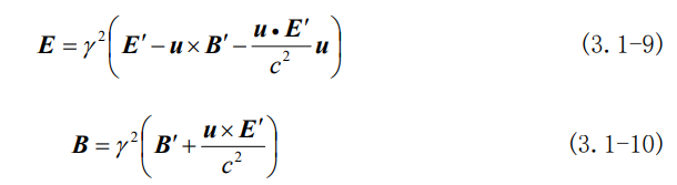
Now, let us prove the following proposition: No need to assume that the speed is very low and the gravitational field is very weak (i.e., no need γ →1), equations (3.1-9) express Faraday's law of electromagnetic induction; Equations (3.1-10) express Ampere's law of total circuit. Let us analyze the simplest case scenario:

Let the K' frame has a velocity u relative to the K frame, with gravitational potential φ. If K measures in K' a magnetic field at rest relative to K' (B ' ≠ 0) and no electric field (E ' = 0), then according to equations (3.1-10) and (3.1-9), we respectively obtain

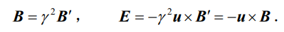
This finding indicates that the K-system observer not only detects the magnetic field B in system K, within the K-system in K but also observes an electric field E in system K. This electric field is precisely generated by the motion of the magnetic field B ' relative to the observer, known as 'moving magnetism generating electricity', which falls under electromagnetic induction phenomena.

To prove that E =- u × B is Faraday's law of electromagnetic induction, take the curl of both sides of the equation:

Since the magnetic field is a field without sources, ∇ · B = 0. Since u is a constant vector, the first and third terms on the right side of equations (3.1-11) are also zero, leaving only the fourth term non-zero. Since E' = 0, B ' is independent of t ', that is

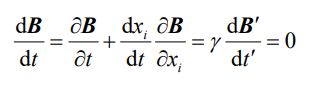
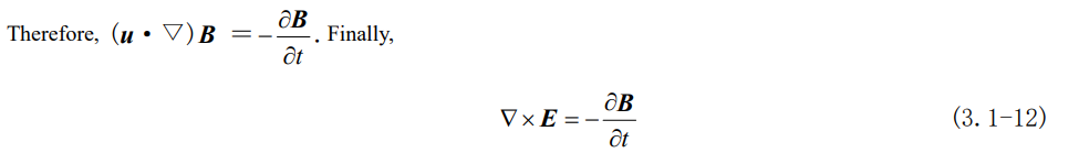
Equations (3.1-12) exactly is the differential form of Faraday's law of electromagnetic induction. In other words, even if the magnetic field moves rapidly within a strong gravitational field, Faraday's law of electromagnetic induction remains applicable.

If the given scenario is changed so that the observer of the SG system K only measures a static electric field (E '≠ 0) relative to the moving frame K', but cannot detect a magnetic field (B ' = 0), then from equations (3.1-9), there is

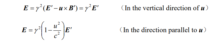
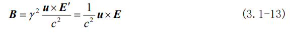
From equations (3.1-10), we know that B ∝ u × E' ∝ u × E. When u // E, B = 0. Therefore, E // u is not considered, leading to

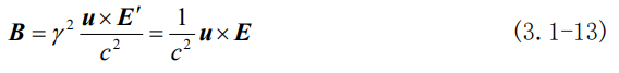
The K system observer not only observes an electric field E in the K coordinate system, but also detects a magnetic field B. This magnetic field is precisely generated by the motion of the electric field relative to the observer, known as 'moving electricity generating magnetism', which falls under the magnetic effect of current. Taking the curl of both sides of equation (3.1-13):

Since B ' = 0, E ' is independent of t ', resulting in

Equations (3.1-16) are precisely Ampere's law of the full circuit. This is sufficient to demonstrate that even when an electric field moves at high speeds within a strong gravitational field, Ampere's law of the full circuit remains applicable.

Using Newtonian Mechanics to Directly Calculate the Precession of Mercury Due to Spacetime Bends

With the Sun's center as the origin O, establish an SG system K(r, φ, t). Using Newton's second law and the law of universal gravitation for Mercury, we have

 

Where G is the gravitational constant, M is the mass of the Sun, r is the distance from Mercury to the Sun, φ is the angle through which the line connecting Mercury and the Sun has rotated, and t is time.

Using any point along Mercury's path as the MF system K' (r',φ',t'), Mercury's motion around the Sun in the background system K can be observed from these points. According to the principle of relativity, all the mathematical expressions of the same form as equation (3.2-1) can be provided:

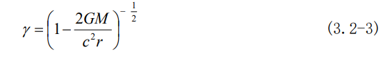
Vividly abbreviated as 'multi-measure-one get same formula'. Each static gravitational field system(abbreviated as the SF system) K' is clearly dual to the SG system K. On the basis of the principle that the roles of the auto-coupling system and the standard system character can be interchangeable, 'multi-measure-one get same formula' is inevitably equivalent to 'one-measure-multi get same formula'. Equation (3.2-2) can also be considered as the observer in the K system, observing the sun and Mercury are all in the background of each K' point and its neighborhood, the dynamical equations for Mercury's continuous motion around the Sun. The Newtonian gravitational potential for these static points is φ = - GM /r, so the spacetime contraction coefficient for each K' frame is given by the following formula:

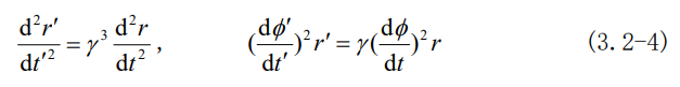
Using four-same spacetime transformations, the transformation relationship between the three-dimensional acceleration of the K system and the K' system can be derived [4](P197):

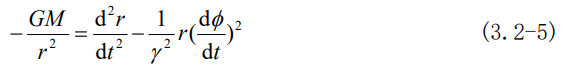
Substitute (2.5-5), (2.5-9), and (3.2-4) into equation (3.2-2) to complete the correction of Newtonian mechanics due to spacetime expansion or contraction:

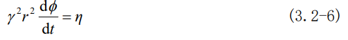
The subsequent steps are not significantly different from those of the classical approach used to derive Binet's equation. However, the conservation law of unit mass angular momentum requires adjustments based on the same proportional contraction in all spatial directions (see equations 3.4-8 in Section 3.4 of this article):

Setting u = 1/r and m = GM / c², equation (3.2-3) can be written as γ = (1-2mu)^-1/2 ≈ 1 + mu. From equations (3.2-5) and (3.2-6), the modified Binet formula corrected for spacetime contraction can be obtained as

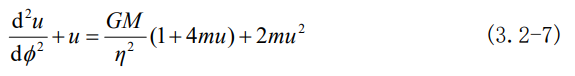
Equations (3.2-7) represent the orbit equation of Mercury around the Sun as observed by the K system observer during a continuous one-by-one observation of those background spacetime K' systems. Unlike the solution of the following orbital equation

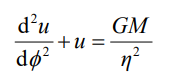
In flat spacetime which is a closed ellipse, the solution of equation (3.2-7) is no longer a closed ellipse but instead, the radius vector sweeps out a small angle each time it completes a revolution around perihelion:

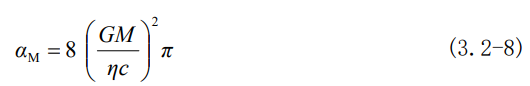
The physical mechanism that generates this angle is as follows: the observer of the K system observes the orbits of Mercury around the sun at each spacetime point K', which should be a closed ellipse, but the condition is that Mercury must be able to move for at least one cycle within each K' system. In reality, Mercury only experiences an extremely short duration at each spacetime point before moving on to the next spacetime point. Therefore, the orbits of Mercury across the entire spacetime background of the Sun, not every single spacetime point K' and its neighborhood complete ellipse, are formed by sequentially piecing together small segments of arc lengths from corresponding parts of closed elliptical curves within each spacetime point's neighborhood that it passes through. Owing to the varying contraction ratios at different spacetime points, the similarity ratios of ellipses in the coordinate systems of each spacetime point differ. Among all the points in Mercury's orbit, the ellipse is smallest in the perihelion coordinate system, and larger at other points, reaching its maximum at aphelion. When Mercury departs from the perihelion, if the arc lengths of each segment it passes through are added, it will naturally be longer than the circumference of the ellipse in the perihelion coordinate system. This is the reason why the actual orbits of planets are not closed, which does not contradict the fact that each point's coordinate system ellipse is closed.

Substituting the data for the sun and Mercury into equation (3.2-8), we obtain α_m = 0.137"/ lap. Mercury orbits the sun at 415.2 laps over 100 Earth years, during which its perihelion advances by 56.78”. From the derivation process of equations (3.2-8), it is evident that 56.78" result from the contraction of the background space observed by an observer in the SG system (i.e., an observer at rest infinitely far from the Sun's center).

However, actual observation values are obtained from observations on Earth. From Earth's perspective, clocks in Mercury's orbit run slower than those synchronized with Earth. During one Mercury cycle, the time difference between the Mercury clock at perihelion and the Earth's clock is as follows:

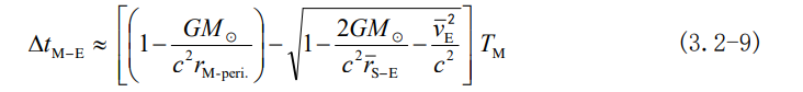
Near Mercury's perihelion, the angle swept by the radius vector corresponding to this time difference is

415.2 laps total is -14.28". The sum of the two items is 56.78" -14.28" = 42.51". This is precisely the total precession of Mercury's perihelion observed from Earth due to time and space contraction, which matches the observed values.

Using Newtonian Mechanics and Huygens' Principle to Calculate the Deflection of Light in the Gravitational Field of the Sun

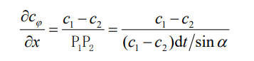
Consider a plane wave of light propagating parallel to the Y-axis. At moment t, its wave front reaches the X-axis. P₁ and P₂ are two points on that plane. The speed of light decreases along the negative X-axis due to changes in the gravitational potential φ, whereas it remains constant along the Y-axis. The speed of light at points P₁ and P₂ is c₁ and c₂ respectively, with c₁ > c₂; after time dt, the distances travelled by light at the two points are c₁dt and c₂dt. According to Huygens' principle, the common tangent Q₁Q₂ of two circles represents the wavefront at time t + dt, as shown in Figure 3.

Figure 3: Diagram of Huygens' Principle of Refraction

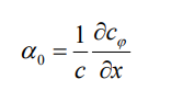
Figure 3, shows that the light is deflected by an angle α towards the negative direction of the X-axis. Given that the distances P₁P₂ are fixed, if c₂ is much smaller than c₁, the deflection angle α of the light will be greater. From the definition of the lateral (perpendicular to the direction of light propagation) gradient of the speed of light, we have

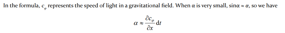
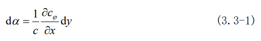
This is the angle at which light deviates while travelling a distance of cdt in the Y direction. Therefore, the angle of deflection per unit distance travelled by light is

Therefore, the angle by which light is deflected when it travels an arbitrary distance dy in the Y direction, that is

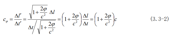
Whether oneself-measure-oneself or one-measure-two, any speed of light defined by dividing local distance by local time is called the intrinsic speed of light. The intrinsic speed of light always equals the speed of light in a vacuum by the SG system observer measured in the SG system, c. To compare the speed of light between the MF system and the SG system, only the following method can be used: compare the time taken for light to travel the same distance in two different systems, compare the distance light travels in two different frames of reference over the same time period, or consider both distance and time in the comparison. This defined speed of light is called the comparative speed of light. When both participate in the comparison, it is called the double-compare speed of light. In the SF system, the expression for the double-compare speed of light is

Assuming that the luminous star, the Sun, and the Earth are all on the Y-axis, the starlight is directed perpendicularly to the X-axis shooting toward the Sun, passes around the Sun, and continues to travel toward the Earth, which is on the opposite side of the Sun, as shown in Figure 4. In the diagram, the circle represents the sun, and it is assumed that the distances from the star to the sun and from the sun to the Earth are both infinitely far. On the Earth observe the motion of starlight, is equivalent to observing it from an infinite distance, i.e., Earth K serves as the standard system. The distance of starlight propagation along the Y-axis is −∞ → +∞.

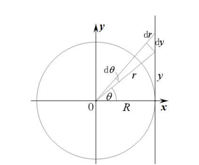
Figure 4: Diagram Showing Starlight Grazing Past the Sun

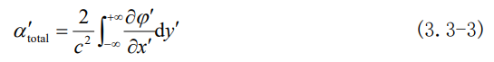
Substituting (3.3-2) into (3.3-1), we obtain the total angle observed by the K observer for the deflection of light in the K system due to the Sun's gravitational field:

Now, select any point on the photon's trajectory as the auto-coupling system K'. Based on the principle of multi-measure-one get same formula equivalent to one-measure-multi get same formula, the K system observer observing the total deflection of light accumulated in each K' system must have the same mathematical form as the above equation:

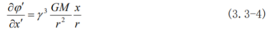
According to Newtonian mechanics, the relationship between the gravitational field strength and gravitational potential is as follows:

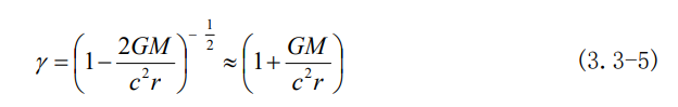
The sun is considered a point mass, so x_M' = 0 in the above equation. Substituting x_m = 0, M ' = γ M , r' = r / γ , and x' = x / into the above equation yields

Equations (3.3-4) express the corrected gravitational potential gradient transformed from the K system to observe the K' system. Since each K' system has a speed of zero relative to the K system, the spacetime scaling coefficient observed by the K system for any K' system is

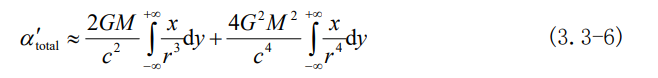
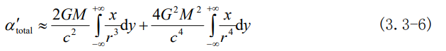
By substituting equations (3.3-4) and (3.3-5), along with dy ' = dy / γ into equation (3.3-3), the cumulative deflection of light observed continuously in K' by K is

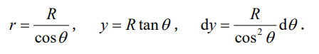
Switching to polar coordinates (r, θ) as shown in Figure 4, allows the closest distance of the light ray to the Sun's center to be the radius of the solar sphere, i.e., x = R:

Substituting them into equations (3.3-6), we obtain

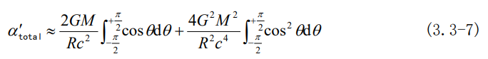
We integrate equations (3.3-7) and substitute the data for solar mass M = 1.893×1030 kg and radius R = 6.95×10 8 m to obtain

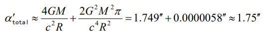
The 5.8" ×10-6 in the formula represents the additional effect on light deflection caused by the correction value for observing the gravitational potential of the Sun in the K' system from the K system observer. This effect is not noticeable because of the weak gravitational pull or high gravitational potential of the sun. 1.75" matches the observed value.

Using Classical Mechanics to Calculate the Radar Echo Delay

In a four-dimensional spacetime coordinate system, if the interval between two infinitesimally close points from the SG system K observed in the K system is defined as

and then substituting (2.5-4) and (2.5-7) into equation (3.4-1), we obtain the interval between two infinitely close points in the arbitrarily MF system K' by the K's observer observations:

In the formula, when the subscript μ = ν, all the coefficients γ are equal to the values of equation (2.5-6),when μ ≠ ν, all the coefficients γ = 0.

According to equation (2.4-2), the coordinate differences multiplied by the physical metric represent the physical quantities. Therefore, in equation (3.4-2), both dx'_μ and dx'_v are multiplied by γ. In equation (3.4-1), both dx_μ and dx_v are also multiplied  by γ, but since γ = 1 in the SG system, it is not written. Therefore, for convenience in writing, the primes on the coordinate differences in equation (3.4-2) can be omitted, and the subscripts can be represented by the same Greek letter. This allows the spacetime interval in an inertial frame to be unified with the line element definition ds² = g_μv dx_μ dx_v in a non-inertial frame (the μ ν potential-speed same working):

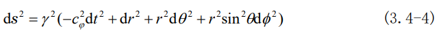
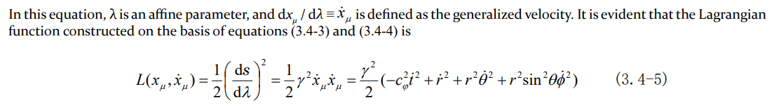
In the formula, the same subscript represents the summation of μ values of 0, 1, 2, and 3. In spherical coordinates(ic_φ t, r, θ,φ), equation (3.4-3) becomes

To determine the time it takes for radar waves to be emitted from Earth, pass by the Sun, reach Mercury, and then reflect back to Earth, we need to know the orbit equation of the photon's motion. For this purpose, we must use Hamilton's variational principle from classical mechanics. That is,

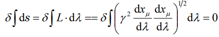
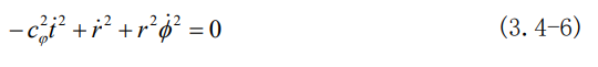
Assuming that radar waves propagate within the plane where θ = π / 2 (dθ / dλ = 0) in spherical coordinates, are emitted from point(r₁,φ₁) and reaching point (r₂,φ₂), then reflect back to (r₁,φ₁); for the photon of the radar wave, since ds = 0, L = 0, equation (3.4-5) becomes

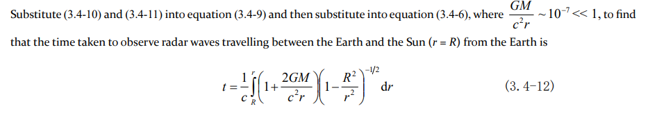
Integrating equations (3.4-12), the result is

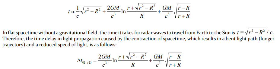
Therefore, the total delay of the radar waves from Earth to Mercury passing through the sun and back to Earth is as follows:

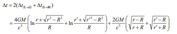
Substituting the values of the Earth-Sun distance r = 1.496×1011 m, the Sun-Mercury distance r'= 5.79×1010 m, M = 1.983×1030 kg, and the Sun's radius R = 6.95×108 m into the above equation, and considering R << r and R << r', the total delay for observing radar echoes that skim past the sun and are reflected by Mercury from Earth (approximately an infinite distance) is obtained:

 

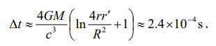
These theoretical calculation values match the actual observed values very well.

Using the Potential-Speed Redshift Formula Derive the Energy-Mass Equation Which Contains the Gravitational Potential

Let K' be an accelerating frame relative to the SG system K along the positive X-axis (with the X' direction aligned with the X-axis ), equivalent to K observing K' in a gravitational field directed along the negative X-axis; a luminous object is at rest in K, with its energy relative to K denoted as E₁ and its energy relative to K' denoted as E₁'. At moment t, the object emits a plane light pulse with energy ΔE / 2 in a direction making an angle θ with respect to the X-axis, while simultaneously emitting an equal amount of light in the opposite direction (π-θ); clearly, the object remains stationary relative to the K system before and after the emission of the light pulse. Let the velocity and acceleration of K' relative to K at moment t be u and a, respectively. The energy of the object after emitting light relative to K and K' is denoted as E₂ and E₂' , respectively. Therefore, in the K system, the energy relationship before and after an object emits light is

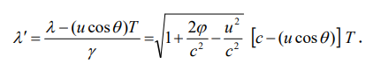
The light source is stationary in the K system and will exhibit the Doppler effect when observed from the K' system. The K' system observer observes that the luminous object is accelerating in the negative direction of the X' axis. At moment t, its velocity and acceleration are - u and -a, respectively. This is equivalent to the observer K' seeing the object in a gravitational field along the positive X-axis (with an equivalent gravitational potential φ < 0 ), so a gravitational redshift effect is also observed by K'. Let light source K be relative to the K' direction of movement at an angle θ with respect to the line connecting the light source to the observer. If K' observes the speed of light in K' to be c, wavelength λ = cT, frequency is ν, and period T = 1/ν, then K' observes the speed of light in K as the double-compare speed of light c '= c / γ ², and the wavelength observed by K' in K is compressed, i.e,

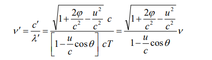
From the relationships among the frequency, wavelength, and speed of light, the frequency observed by an observer in K' for the light emitted by a source in K can be determined as

This is the potential-speed redshift formula derived purely from a physical perspective, comprehensively taking into account both Doppler redshift and gravitational redshift. Since the light source is fixed in K, ν' is the emission frequency of the light source, also known as the intrinsic frequency, and ν is the reception frequency in K'; thus, we obtain

 

Therefore, the frequency of light waves emitted in two opposite directions by the light source in the K system, as measured by the K' system, separately is

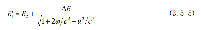
Then, by the energy of the photon E_photon = hν, the energy relationship of the K system object before and after light emission in the K' system can be obtained as follows:

Taking hν_intrin = ΔE / 2 into account, we obtain

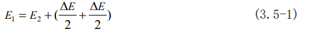
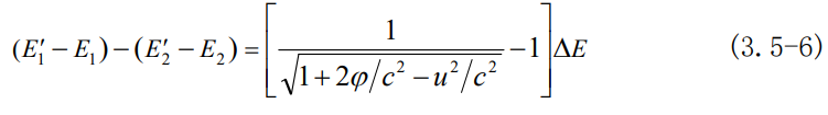
Subtracting equation (3.5-1) from equation (3.5-5), we obtain

 

Before and after the object emits a light pulse, observer K observes that its energy has decreased by ΔE and that the object has no kinetic or potential energy before or after emitting light. However, observer K' observes that, in addition to the energy lost due to the emission of the light pulse, the object's kinetic and gravitational potential energies change both before and after it emits light. Therefore, for K', the difference (E'-E) is different from the object's mechanical energy only by a constant C, where C represents the total energy of all other forms of energy in addition to mechanical energy. Ignoring higher-order small quantities, this constant C is the object's rest energy. On this basis, we set

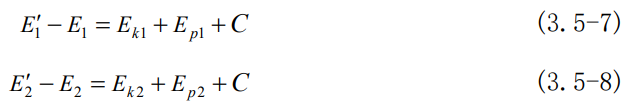
By substituting equations (3.5-6) into (3.5-7) minus (3.5-8), we obtain

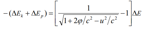
Expand expression (1+2φ/c²-u²/c²)1/2 By neglecting higher-order infinitesimals in cases where φ << c² and u << c, we obtain

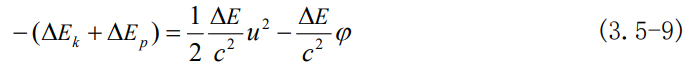
The two terms on the left side of equation (3.5-9) should correspond respectively to the two terms on the right side, i.e.,

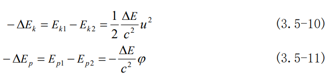
Equations (3.5-10) show that the kinetic energy of an object after emitting light is less than its kinetic energy before emitting light. Compared with the K' system, the speed of the objects is all -u before and after light emission, so the reduction in the object's kinetic energy is confirmed to be independent of velocity. From the definition of kinetic energy E_k = mv² /2, we know that the change in kinetic energy is ΔE_k =Δm(-u)² /2. Therefore, a decrease in kinetic energy can be caused only by a reduction in the mass of the object.we obtain

Following the same logic, the change in gravitational potential energy should be unrelated to changes in gravitational potential (where the equivalent gravitational potential at the same position remains constant) and related only to changes in the mass of the object. Equation (3.5-11) indicate that the gravitational potential energy of an object after emits light is greater than its gravitational potential energy before emits light. From the previous analysis, it is known that in this example, φ < 0. Therefore, from the definition of gravitational potential energy E_p = mφ, an increase in gravitational potential energy is also caused by a decrease in mass (since the smaller the mass is, the less one loses the gravitational potential energy). We obtain

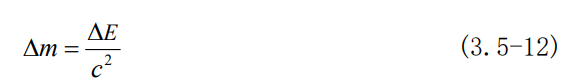
First, we merely assumed that an object emitted light energy ΔE; the final result, however, was that the object's mass decreased by ΔE/c². This obvious cause-and-effect logic reveals a fascinating connection between energy and mass:

Equations (3.5-14) describe the relationship between the change in energy and the change in mass of an object, whereas E₁= m₁c^₂ and E₂ = m₂c^₂ represent the correspondence between energy and mass. Without the subscript, it becomes the universal  mass-energy equation:

In equations (3.5-12), the mass related to an object's kinetic energy is called the inertial mass m_I by convention; whereas in equations (3.5-13), the mass related to an object's gravitational interaction is referred to as the gravitational mass m_G . After energy ΔE is emitted with a light pulse, both decrease by the same amount ΔE/c². Therefore, from equations (3.5-12) and (3.5- 13), we have Δm_I = Δm_G , that is

This is none other than the famous Einstein equivalence principle. Now, it is no longer an assumption but rather a necessary outcome of theoretical derivation.

The Application of the Four-Same Spacetime Transformation Formula in the Flight of Cesium Clocks and the Reduce Frequency Experiment of GPS Satellite Clocks

Cesium Atomic Clock Global Flight Experiment

To test the time dilation effect, in 1970, Hafele from the University of Washington in the United States designed and conducted an experiment involving cesium atomic clocks on a global flight, as shown in Figure 5. The solid line circle represents the Earth's equator, with R being the Earth's radius. The Earth rotates around its axis O from west to east at an angular velocity of ω. Two groups of identical cesium atomic clocks were calibrated and synchronized; one group was placed on the ground, while the other was placed on an airplane. Initially, both groups of clocks are located at point P on the Earth's equator. The airplane then takes off and flies at an altitude of h. After circling the equator once and landing back at P, the time recorded by the stationary clock on the ground is compared with that recorded by the clock on the plane. Let τ₀ represent the time measured by the ground clock, and let τ represent the time measured by the clock on the airplane. When the plane flies eastwards, it is denoted as τ_E, and when it flies westwards, it is denoted as τ_W.

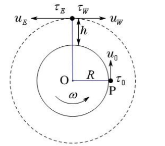
Figure 5: Diagram of the Global Flight Experiment with Cesium Atomic Clocks

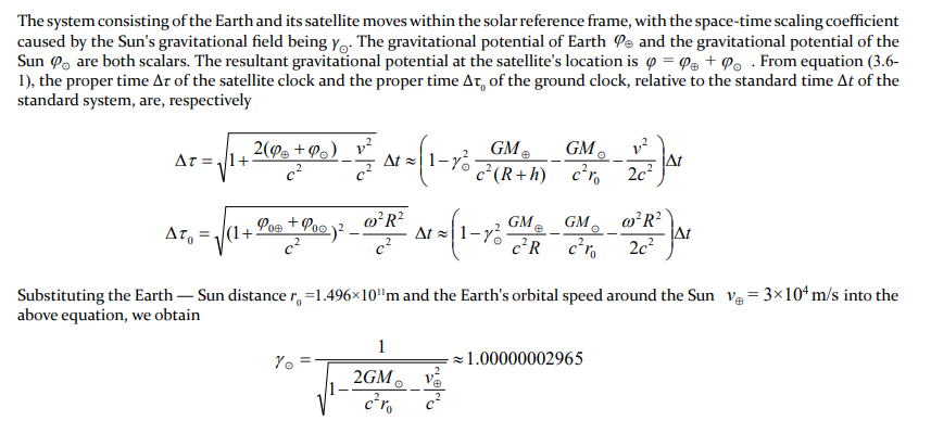
Hafele assumed that the Earth rotates at a constant angular velocity ω (spins) within a nonrotating reference frame K, where there exists a gravitational field identical to that of the Earth's gravitational field. He is precisely based on the K coordinate system and calculates the difference between the reading of an atomic clock after one circumnavigation flight and the reading of an atomic clock on the ground. Its theoretical basis includes the time dilation formula from special relativity and the approximate formula from general relativity, which states that the difference in the rates of two clocks is proportional to the difference in their gravitational potentials in weak gravitational fields. First, each effect is derived independently, and then forced together with a linear relationship.

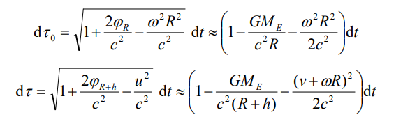
Now, according to the principle of 'potential-speed same working', replacing the Lorentz spacetime contract coefficient with equations (2.5-6), eliminates the need for the subjective assumption that the two effects add linearly. Instead, it integrates both effects into one seamless process. I.e., in general cases, the relationship formula between the two what the standard system (the SG system) measures the MF system’s time dτ, with the SG system measures its own time dt, can be written directly:

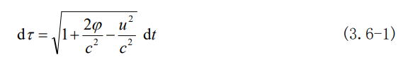
Applying equation (3.6-1) to the ground clock and the airplane clock, we obtain

By substituting GM_E = gR² into the above equation, and ignoring the occasional errors of the aircraft clock deviating from the equatorial plane and eastwards direction, we obtain the difference in the readings of the two clocks after one circumnavigation. It is

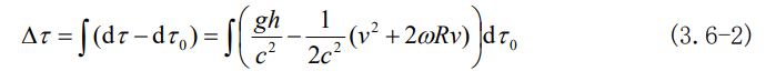
The relevant data are substituted into the calculation, and the final result is as follows: τ_E - τ₀ =-59ns and τ_W - τ₀ =273ns. These findings are consistent with actual observations.

Experiment on Reducing the Frequency of GPS Satellite Clocks

Assuming that a GPS satellite is 20,000 km above the Earth's surface and orbits at a speed of 14000 km/h, the clock frequency on the satellite must be adjusted to 10,229,999.99545 Hz when the standard clock frequency is set to 10.23 MHz. Otherwise, the positioning error would exceed 11 km in a day.

Substituting the relevant data (with gravitational acceleration g at the Earth's surface taken as 9.8 m/s²), the result of the calculation is

If the ground clock measures 1 day as Δτ₀ = 86400 s, then the satellite clock measures 1 day as Δτ = 86400.0000384566s, which means that the satellite clock is faster than the ground clock by 38.457μs/d. Therefore, the satellite clock must be slowed by 38.457μs/d to synchronize with the ground clock. That is, the satellite clock frequency must be 38.457μs/ 86400s, which is 4.451×10^-10 times lower than that of the ground receiver; in other words, the satellite clock should oscillate 4.451×10^-10 fewer times per second than the ground clock. When the ground clock frequency is set to 10.23 MHz, the satellite clock frequency must be reduced by 10.23 × 4.451 × 10 ^{- 10} MHz = 0.0045534Hz, resulting in a frequency of 10229999.995447Hz. This approach is more accurate than calculating the sum of the two effects separately and reducing the satellite clock frequency by 0.0045502Hz, which will undoubtedly contribute to improving the precision of satellite positioning.

Solving for the Muon Lifetime in an Accelerator Via the Four-Same Spacetime Transformation Formula

In 1966, Farley and colleagues conducted an experiment using a high-energy accelerator, comparing the lifetimes (or decay rates) of muons when they travelled at the same speed in straight lines versus circular paths, and claimed that the experiment confirmed with 2% precision that the decay rate of muons is independent of acceleration [5] (P14). However, the following derivation shows that this experiment does not prove that the muon's lifespan is independent of acceleration.

All the circular motion experiments share a common feature: their centripetal acceleration a_n = ω² r = v² /r = ωv. When ω = 0 or v = 0, it is certain that a_n = 0. This finding indicates that circular motion is not an accelerated motion where acceleration and velocity are independent of each other. Therefore, within the spacetime scaling coefficient γ, once the effect of motion has been considered, it is no longer necessary to consider the acceleration effect or the equivalent centrifugal force field effect, and vice versa.

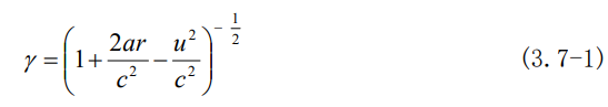
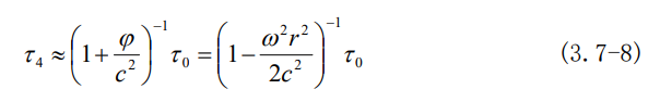
If the acceleration at a radius r in circular motion is a, then the gravitational potential φ at that point can be written as φ = ar . Equations (2.5-6) can be written as

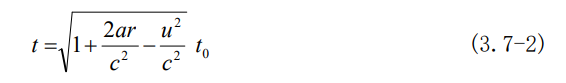
The relationship between that the standard system K measures the time (or clock frequency) t in the auto-coupled system K' and the standard system K measures the time t0 in the K system, is

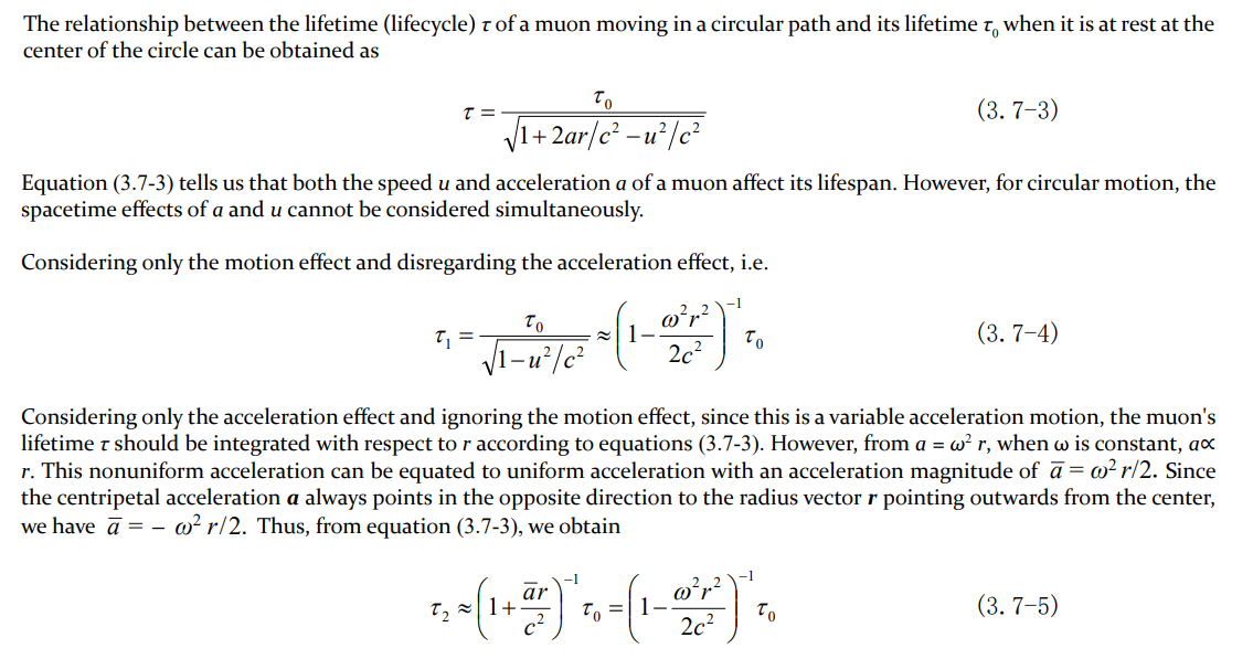
If a muon moves with uniform linear motion and its speed is exactly equal to the tangential speed of circular motion, i.e., u = r ω, then from equation (3.7-3), the muon's lifetime can be obtained:

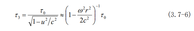
For muons undergoing circular motion, the lifespan τ2 considering acceleration effects is exactly equal to the lifespan τ1 without considering acceleration effects. The lifespan τ3 of a muon moving at a constant velocity in a straight line is exactly equal to the lifespan τ1 of a muon undergoing circular motion if their speeds are the same. However, the above relationship does not prove that acceleration has no effect on the muon's lifespan, because τ3 is also equal to τ2, indicating that the effect of accelerated motion on the muon's lifespan is the same as the effect of uniform linear motion on the muon's lifespan. This demonstrates that experiments related to circular motion cannot prove that 'acceleration does not affect the fast and slow of clocks' or that 'acceleration does not affect the properties of standard measuring rods'.

The equivalence principle is one of Einstein's deepest insights, stating that acceleration within an accelerating frame affects spacetime in the same way that a gravitational field affects spacetime within its field, in terms of their effects. The centripetal acceleration of circular motion as is treated an inertial force field pointing outwards from the center, with a field strength of

When ω is constant, g ∝ r, this nonuniform field can be considered a uniform field with strength g = g / 2; the gravitational potential at a distance r from the center is φ =-g r =- ω²r² / 2. For circular motion, if acceleration a is considered, velocity u cannot be considered. Similarly, if the inertial force field's potential φ is considered, the speed u cannot be considered. Therefore, from equations (3.7-3), we can determine that the lifespan of muons in an inertial force field is

 

Revisiting Quasars and the Expansion of the Universe Via the Potential-Speed Redshift Formula

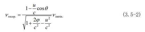
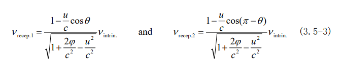
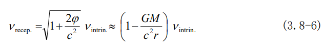
If the light source is stationary in the auto-coupling system K', then the frequency ν_recep. received by an observer in the reference frame K is related to the intrinsic frequency ν_intrin. emitted by the source in the K' system by reversing equation (3.5-2):

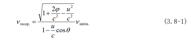
In the formula, u and φ represent the speed of the light source relative to K and the gravitational potential, respectively; θ is the angle between the line connecting the light source to the observer and the direction of the light source's movement. θ = 0 and θ = π indicate that the light source is approaching and moving away from the observer, respectively.

Quasars Phenomena

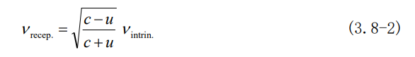
If the gravitational field at the source of light is not considered, i.e., φ = 0, then equation (3.8-1) becomes the Doppler redshift formula (θ = π):

If the relative redshift amount of light waves via wavelength or frequency is defined as

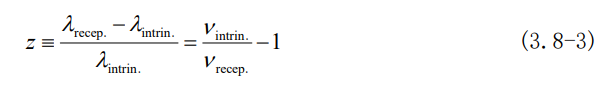
Then, from equations (3.8-2) and (3.8-3), the recessional velocity of the quasars can be obtained:

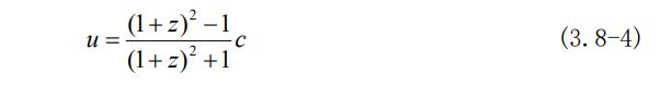
By substituting the redshift amount z = 6.3 of the quasar SDSS J0100+2802 discovered by Wu Xuebing's team at Peking University into equation (3.8-4), we obtain u = 0.96c. It is difficult to imagine such a massive stellar system moving away from us at nearly the speed of light.

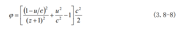
On the other hand, if we consider that redshift is solely caused by a gravitational field, treating the entire quasar as a sphere with radius R and mass M, using the pure temporal component of the Schwarzschild metric equation, we can derive the gravitational potential at the surface of the quasar: [5] (P153)

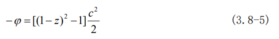
Substituting z = 6.3 into equation (3.8-5), we obtain the following for the quasar: −φ = GM/R =13.5c². What does this mean? More than 200 years ago, P.S.Laplace used Newtonian mechanics to calculate the conditions for celestial bodies to become dark stars, which were the same as those derived by Schwarzschild more than 100 years later using Einstein's field equations for black holes, i.e., R ≤ 2GM / c². Rearranging this equation gives GM / R ≥ 0.5c². Using equation (3.8-5), we find that GM / R = 13.5c², far exceeding the minimum condition for becoming a black hole, GM / R = 0.5c², so it should have already turned into a black hole long ago. However, we can still observe it on Earth. Therefore, the gravitational redshift theory of general relativity alone cannot also explain the enormous redshift of quasars.

However, for equation (3.8-1), if we ignore the motion of the light source (u = 0) and only consider it to be within a gravitational field, then

From equations (3.8-6) and (3.8-3), we can obtain

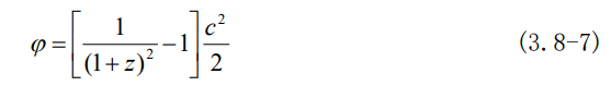
Substituting z = 6.3 into equation (3.8-7), we obtain φ = −0.4906c2. Since −0.4906c2 > −0.5c2, the equipotential surface of this gravitational potential of the celestial body is greater than that of a dark star (black hole) and certainly does not lie within its boundary. Even without considering the movement of quasars, they can be easily observed on Earth.

In the real universe, completely stationary celestial bodies do not exist. Notably, celestial bodies that do not produce any gravitational field also do not exist. When both motion and gravitational effects are considered simultaneously, extreme scenarios such as quasars moving at speeds close to the speed of light or gravitational potentials approaching black hole conditions do not occur. This indicates that problems that cannot be solved separately via the Doppler redshift formula and the gravitational redshift formula can be solved via the potential-speed redshift formula. This finding also indicates that Hafele's approach in Section 3.6 of first solving using the time dilation formulas of special and general relativity separately, then linearly adding them together, lacks a theoretical basis.

Determining Factors of the Spectral Redshift of Celestial Bodies Via the Potential-Speed Redshift Formula

Ignoring the movement of the light source, according to equations (3.8-6), if the gravitational potential at the observer's location is greater than that at the light source, the observed phenomenon is redshifted; conversely, it is blue shifted. This is consistent with the gravitational redshift formula of general relativity, which has been confirmed by the Mössbauer experiment and the solar gravitational redshift experiment; further elaboration is unnecessary here.

When both the motion of the light source and the gravitational effects at the light source are considered simultaneously, the frequency shift observed by the K system observer is significantly different from what American astronomer V. M. Slipher imagined. Since the gravitational potential of an observer on Earth is always greater than that of a light-emitting celestial body, we can observe only the redshift effect caused by gravity. Equation (3.8-1) shows that when the gravitational potential at the source of light is low enough, regardless of which direction the light-emitting celestial body moves, the observed combined effect on Earth is still redshifts. Here, we specifically discuss the case where θ = 0, which is the situation most prone to blueshift (i.e., when the celestial body is moving towards Earth). From equations (3.8-2) and (3.8-3), the relationships among u, φ, and z can be derived. This relationship is

According to equations (3.8-8), even if SDSS J0100+2802 approaches Earth at a speed of u = 0.96c, a redshift amount of = 6.3 can be observed on Earth with only a gravitational potential φ = −0.0392c² at its surface light source. Even under conditions where celestial bodies travel towards Earth at such extreme speeds (Note: This is not the scenario of being far from Earth that Slipher mentioned!) and their surface gravitational fields are not particularly strong, they can still produce this extreme redshift. This proves that the redshift of the galaxy spectra does not necessarily mean that the galaxies are moving away from Earth. Unless the emitting celestial bodies do not generate gravitational fields, they are not located within other gravitational fields.

In the real universe, the light emitted by galaxies of all sizes, especially distant ones, that can be observed by humans must come from areas where stars are more densely packed within those galaxies. If the gravitational potential is φ ≤ −0.001c² (which can easily be satisfied by a galaxy), according to equations (3.8-8), as long as the speed of the galaxy towards Earth does not exceed 0.001 times the speed of light, the redshift amount observed on Earth for that galaxy will not be less than 0.001 (approximately 470 times the redshift of the Sun's surface). If galaxies move away from Earth at any speed, it will only increase the redshift amount.

From this perspective, when observed from Earth, the spectra of the vast majority of galaxies in the universe are all indeed redshifted. However, the primary cause of redshift is not the motion of celestial bodies but rather the gravitational potential at the point where they emit light. It is evident that relying solely on the special Doppler effect to infer that galaxies are all receding each other on the basis of their spectral redshift does not consider the gravitational influence on the galaxies. Once judged by the potential-speed redshift formula, the hypothesis of cosmic expansion on the basis of the recession of galaxies immediately loses its theoretical foundation. The accelerated expansion of the universe would be impossible to discuss, and dark energy would lose its necessity. The Big Bang theory of cosmic origin also faces severe challenges.

Let us revisit the logic behind determining that quasars have extremely high brightness: from the high redshift amount z, it is inferred that quasars have high recessional velocities u. Using Hubble's law d ∝ u, it is further inferred that they are at great 2 distances d. Finally, according to the astronomical rule that apparent brightness L_V ∝ L_G / d , when L_v is constant, from L_G ∝ d² it can be inferred that they have extremely high luminosity L_G . If a high redshift does not correspond to a high recessional velocity, this logical chain clearly breaks.

Let us imagine another scenario: if quasars are assumed to be stationary relative to the Milky Way, their speed relative to Earth would be the sum of the speed of the solar system relative to the Milky Way and the speed of Earth relative to the solar system, approximately u = 0.001c. According to equations (3.8-8), as long as the gravitational potential φ at the surface where the quasar emits light is approximately −0.4906c², it ensures that the redshift amount observed on Earth is z = 6.3. Compared with the speed of 0.963c calculated without considering gravity, the speed is reduced by approximately 1000 times, which means that the distance to Earth decreases from 1.28 billion light-years to 12.8 million light-years; its luminous brightness decreases by a factor of 106. According to equations (2.5-6), owing to motion and being in a gravitational field (the gravitational potential of a spherical celestial body within its own gravitational field, after integration, is half of its surface gravitational potential), the radius of the celestial bodies contracts by a factor of γ = 1.43, which means that the surface area of the celestial body shrinks by a factor of 1.43², implying that the L increases by a factor of 1.43². After this part is subtracted, the luminosity of the quasar decreases from 430 trillion times the brightness of the sun to 215 million times the brightness of the sun. Compared with ordinary galaxy, which often contains hundreds of billions of stars, even a small galaxy would have this level of brightness as normal. In summary, there is no need to consider quasars as extraordinary celestial bodies, for either high redshift amount or high brightness; they can all be reasonably explained via the potential speed redshift formula.

NCSC Physics Theoretical Prophecy and Their Astronomical Verification

A large Number of Hidden Ordinary Stars are a Significant Source of Dark Matter

Since the 1920s, a series of astronomical observations, particularly galactic rotation speed curves, have confirmed that there is several times more dark matter in galaxies than visible matter. Early speculation suggested that dark matter consisted of massive dense celestial bodies made of conventional matter, such as black holes, and neutron stars. However, because the total amount of these objects was too small, it was hypothesized that there must be a large quantity of nonbaryonic dark matter. Despite extensive efforts over nearly a century, nonbaryonic dark matter has yet to be detected.

We can return to the starting point and imagine that the hidden matter, apart from massive compact objects, consists of ordinary nondense celestial bodies. However, this requires rigorous a mathematical proof, which is provided below:

Unlike black holes, these celestial bodies can emit or reflect photons outward. However, when observed from Earth, the received light wave frequency becomes zero due to infinite redshift, i.e.,v_recep = 0. From equation (3.8-1), since ν_intrin ≠ 0, it follows that

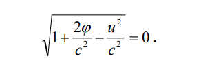
Solving this equation yields: the range of gravitational potential values for the light source that makes ν_recep. = 0 when u is determined, i.e.,

Alternatively, if φ is determined, the range of light source motion speeds that make ν = 0 is as follows:

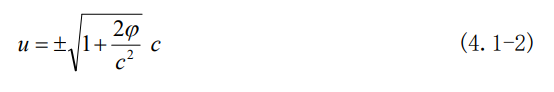
Equation (4.1-1) shows that when u = 0, φ = −0.5c² , this equipotential surface is precisely the infinite redshift surface of a stationary celestial body; when u takes a positive value, i.e., when the celestial body moves away, φ > −0.5c² , which indicates that a receding celestial body more easily becomes a hidden ordinary star; when u takes a negative value, i.e., when the celestial body moves towards us, φ > −0.5c² , which indicates that an approaching celestial body is less easy more to becomes a hidden ordinary star.

Some celestial bodies, although they themselves do not meet the aforementioned criteria for invisibility, can help the celestial bodies around them become hidden. For example, the gravitational potential at the surface of a single stationary star (whose radius is R) is as low as −0.45c² , the redshift value can be calculated from equations (3.8-8) as z = 2.3, which is a finite redshift, indicating that this star does not have enough gravitational potential to become a hidden ordinary star. At a height of 0.3R above its surface, the gravitational potential is −0.3461c² , which is calculated from equation (4.1-2), for celestial bodies orbiting around it at this height (ignoring their own gravitational potential), the speed required for hiding should reach 0.555c; According to Newton's law of universal gravitation and the second law of motion, the orbital speed at this height is 0.558c, which is greater than the speed needed for hiding. Therefore, any celestial body on this orbit will inevitably be invisible. Furthermore, it can be concluded that all celestial bodies within the range R < r < 1.3R around this star are clearly invisible, and this area is commonly referred to as the 'dark matter halo' region. If there are many invisible celestial bodies within this halo area, the range of the dark matter halo significantly increases.

For example, in some binary or multiple star systems, individual stars may not be invisible when stationary, but when they rotate around their common center of mass, some or all of them might become invisible stars. The closer they tare, the higher their operational speed and the greater their gravitational potential overlap, making it easier for them to become invisible stars. If they remain visible even when they are close to each other in a region far from other celestial bodies, when they enter the gravitational field of other celestial bodies (superimposing their gravitational potential), they may become invisible stars. In addition, in the vast universe, from individual stars to binary systems, star clusters, galaxy clusters (groups), and superclusters, gravitational potential and velocity accumulate layer by layer, celestial bodies that do not meet the criteria for invisibility will eventually become scarce. This is why dark matter constitutes the majority whereas visible matter makes up a smaller portion. Such theoretical prophecies align highly with extensive actual observations made by astronomers from early times to recent years.

In a galaxy, around each massive star cluster, there are several smaller clusters or scattered groups of stars that are hidden, filling what appears to us as empty space. If all these invisible celestial bodies were made visible, we would see the entire galaxy filled with densely packed objects, with the distribution density increasing closer to the center and decreasing towards the edges. Therefore, the mutual constraints between celestial bodies within the central region are very strong, becoming weaker as one moves outward, as a result, the entire galaxy resembles a cohesive entity that transitions from within outwards through states similar to solid, liquid, and gas. When the entire galaxy rotates around its central axis, in the 'solid' part near the axis, the speed of the celestial bodies increases linearly with distance from the axis; when the entire galaxy enters the 'liquid' and 'gas' regions, owing to the gradual decrease in the constraints between different parts of the celestial bodies, their speeds no longer increase significantly with distance, but they also do not decrease inversely proportional to the square root of the distance, as seen with planets in our solar system. Instead, they follow Vera Rubin's 'galaxy rotation curve'.

Unlike the absolute invisibility of black holes, these soft invisible celestial bodies are relatively invisible. They appear invisible when observed from Earth, but they may not be invisible when observed from closer distances where the gravitational potential is low enough.

Astronomical Observational Evidence of the Hidden Ordinary Stars

Currently, numerous astronomical observations have confirmed the theoretical prophecy of ordinary star invisibility. For example, a team led by astronomer Beatriz Villarroel from Stockholm University in Sweden observed in 2016 that a star mysteriously 'disappeared' from a photograph of the constellation Lupus taken by the united states naval observatory (USNO) on March 16, 1950. In the following years, further observations not only failed to locate the star that had 'disappeared' in the photograph but also revealed approximately 100 point sources (i.e., celestial objects) visible only during that era within the red band marked by USNO, these too mysteriously vanished from the DR-1 images. Therefore, researchers unanimously believe that such regions where stars mysteriously disappear should exist abundantly in the universe. What they refer to as 'disappearance' is actually when celestial bodies become invisible as they move into areas of lower gravitational potential. Another example is Boyajian's Star, designated KIC 8462852, which experiences irregular periodic dimming of up to 22%. If we assume that the obscuring body is an irregularly shaped cluster of multiple stars that rotate on its own axis, and periodically move in front of the luminous object's dark matter halo region, its obscuring effect easily matches the recorded light variation curve. Furthermore, explaining the 'bullet cluster phenomenon' using the abundance of invisible stars within galaxies is more consistent with actual observations than using hypothetical nonbaryonic dark matter.

Conclusion

Physics evolved from the SCS stage to a more advanced NSCS stage, which is an inevitable path for the development of physics. Failing to realize the objective existence of two stages and their differences can lead to misjudgments when using SCS thinking to analyze NSCS physical phenomena. An important and fundamental example is: Newton's absolute theory of space and time, which emerged during a period when observers and backgrounds shared the same coordinate system, whereas the theory of relative space and time became a topic of discussion only after physics had advanced to the NSCS stage. During the SCS stage, without defining time and space as Newton did, it is impossible to describe the laws of motion of objects. In the NSCS Phase, the observer from the standard system directly observes the space and time of the MF system, using the spacetime standards from the standard system (i.e., the SG system). When the observer indirectly observes the motion of the particles in the MF system via the MF coordinate system, the spacetime standards from the standard system are still employed. This indicates that even at the NSCS stage, there is no need to redefine time and space. Relative time and relative space only have physical significance when defined via absolute time and absolute space, under the condition of the one-measure-two. Moreover, with respect the same motion and gravity, within the same system they only produce mechanical effects, whereas between different systems they only produce spacetime effects. Two spacetime conceptions that have all no intersection on the scope and applicable conditions cannot be compared in terms of superiority or inferiority. After the differences between the SCS and the NSCS are fully recognized, combining classical physics from the SCS phase with spacetime theories from the NSCS phase, this forms the modern physics of the NSCS stage. The fusion of the two merely adds one more step of the four-same spacetime transformation, it is identical to the SCS phase in addition to this.

To achieve organic integration of classical physics and space-time theory, it relies on the inherent compatibility and symbiotic qualities of space-time theory with classical physics, rather than modifying classical physics to accommodate incompatible space- time theory. Therefore, the task of this paper is to explore spacetime theories between different systems that are compatible with classical physics, without crossing boundaries to touch upon fundamental physical laws that belong exclusively to the same system studied by classical physics. It is obvious that only the theory of the four-same spacetime transformations possesses the required qualities.

For example:

• The space isotropic can overcome the three-dimensional difficulties in the integration of classical physics and spacetime theory.

• The potential-speed same working can bridge the natural chasm between motion and gravity for their mechanical effects; thus, there is no need to study their spacetime effects separately. Even if gravity is isolated for separate studies, the conclusions obtained are only about the spacetime effects of gravity (the SG system observer observes the gravitational field, and the spacetime is curved), and fundamentally cannot replace nor be used to negate the mechanical effects of gravity within the same system (the law of universal gravitation).

• The coupling-standard isomorphism is one of the two conditions for extending classical physics to the NSCS stage, whereas the space-time same-change and the space isotropic are the prerequisite conditions for the coupling-standard isomorphism. After entering the NSCS phase (observing astronomical phenomena from Earth are typical NSCS type), one often encounters problems that cannot be solved by classical physics; they tend to believe that this is due to inherent flaws in classical physics itself, without realizing that it is because they have not kept up with suitable theories of space and time, or have simply used spacetime theories as fundamental physical laws.

The core of spacetime theories that can coexist harmoniously with classical physics is the law of four-same spacetime evolution; its experimental basis lies in the transverse Doppler of light and gravitational redshift effect. The theoretical foundation for deriving the four-same spacetime transformation formula is the measurement principle of one-measure-two, and the logical support behind the measurement principle of one-measure-two comes from the nature original commandment that only the background coordinate system can serve as the reading coordinate system (relying on the measurement principle or this original commandment, only can be made Figure 2). This nature original commandment is almost a common-sense axiom in both life and experimentation. For example, when an audience watches a play, they must use the stage as the basis for judging the actors' movements. If each audience member uses their own coordinate system, different audiences will give different judgments on the same actor's movements, making it impossible to achieve the intended performance effect. The reason is that the stage serves as the background coordinate system for actors' performance, whereas the coordinate system of the audience, is not the background coordinate system. The various physical phenomena that naturally form also have their temporal and spatial backgrounds that are naturally formed. Therefore, during the NSCS phase, while the observational coordinate system can still be chosen arbitrarily, the background coordinate system used for measurement and reading cannot be arbitrarily designated by humans. This is the origin of the term 'nature original commandment'. Observers in different states of motion and gravitational fields, observing the same movement of the same background coordinate system, except for differences in the ratio of spacetime changing, will all give the same description of the fundamental physical laws that the movement follows. This is the underlying logic of the principle of relativity. In contrast, if observers in different states give varying descriptions of the same motion, then there cannot be universally accepted fundamental physical laws, and thus physics would not arise. This proves that the principle of relativity is an axiom at the metaphysical level. The nature original commandment (only the background coordinate system as the reading coordinate system) with the principle of relativity are fundamentally equivalent. Those who have not awakened the SCS and the NSCS consciousness cannot perceive this equivalence relationship, and therefore cannot develop a spacetime theory that coexists harmoniously with classical physics. Consequently, they cannot extend classical physics into the NSCS realm.

References

1. Einstein, A. (2013). Relativity: The Special and The General Theory - A Popular Exposition. Translated by Bu Tian Zhang. Beijing: Commercial Press.
2. Canbin, L., & Bin, Z. (2009). Introduction to Differential Geometry and General Relativity.
3. Zhang, Y. Z. (1979). Experimental foundations of special relativity.
4. Jian-Xun Zhang. (2019). Spacetime Metric Analysis. Wuhan: Wuhan Publishing House.
5. Liu, L., Zhao, Z. (2004). General Relativity (Second Edition). Beijing: Higher Education Press.
6. Feynman, R. P. (2004). Six Not-So-Easy Pieces: Einstein's Relativity, Symmetry, and Space-Time. Translated by Zhou Guo-Rong. Hunan: Hunan Science and Technology Publishing House.