The Clock of Regimes: Matrix-Analytic Solutions for Continuous-Time Survival in Discrete HMMs using the R KRONX Package*

Introduction

Regime-switching models serve as a foundational framework for capturing the time-varying dynamics of asset returns. The standard approach—pioneered by Hamilton (1989) and adapted for financial applications by Rydén et al. (1998)—characterizes log returns as realizations from a Kcomponent mixture model, where transition probabilities are governed by a latent Markov chain. While several R packages implement this architecture—notably depmixS4 (Visser and Speekenbrink, 2010), HMM (Himmelmann, 2010), MSwM (Sánchez-Espigares and López-Moreno, 2021), and the financially-focused fHMM (Oelschläger et al., 2023)—their primary utility lies in state estimation and parameter inference. Consequently, while these tools identify the current regime of a time series, they offer little insight into the duration of state residency or the system’s proximity to structural absorption and ruin.

This paper introduces the KRONX R package which fills that gap. The package takes the estimated transition matrix from a fitted Hidden Markov Model (HMM) and converts it into a survival-analytic operator system that characterizes the residence geometry and finite-horizon fragility of the Markov chain. The intellectual foundation draws from compartmental analysis, and compartmental systems mean residence times (Berman and Schoenfeld, 1956; Hearon, 1972, 1981; Eisenfeld, 1981; Covell et al., 1984; Linares et al., 1987, 1988; Jacquez and Simon, 1993; Jacquez, 2002). The central object in the KRONX R package is a continuous-time generator and its associated resolvent operator,N= −K^−1, which measures expected cumulative time spent across regimes. This operator-based formulation permits a structural decomposition of persistence beyond one-step transition probabilities and connects regime dynamics to survival analysis through state-dependent hazard rates (Kleinbaum and Klein, 2012; Gao and He, 2025). By integrating hazard rates, the model allows for state-dependent exit and connects regime dynamics to survival analysis and tail risk.

This paper is structured as follows. Section 2 provides the necessary background and a review of the relevant literature. Subsection 2.1 formalizes the open system dynamics of the COR model, while Subsection 2.2 characterizes its fundamental matrix geometry. The transition to a survival analysis framework is developed in Subsubsection 2.2.1. Subsection 2.3 is devoted to the directional change (DC) framework and its alignment with the COR framework. Subsubsection 2.3.1 discusses how DC may be viewed as an event-time observation layer feeding the COR model. Subsubsection 2.3.1 discusses DC thresholds and how they may behave once persistence accumulates. Subsubsection 2.3.3 discusses how DC-derived indicators may be integrated with the COR framework. Subsubsection 2.3.4 discusses the synthesis of DC, HMM, and COR models. Subsection 2.4 discusses the COR framework’s move beyond the limitations of Gaussian assumptions. Subsection 2.5 discusses the COR framework’s inherent Bayesian interpretation.

Background and Literature Review

In Hamilton-style regime switching:

                                                                                S ∈ {1, . . . , K}

represents the hidden regime process. The clock of regimes (COR) model accepts this hidden regime structure, but argues that transition probabilities alone are insufficient to describe systemic fragility. Classical HMMs focus on:

                                                                           P(S_t = j | S_t−1 = i) = a_{i j}

while COR asks how long does risk survive inside a regime architecture once hazard and persistence interact? This leads to the COR operator chain:

                                                                             A → Q → K → N

where:

•A = HMM transition matrix,

•Q = diag(1 − ) A = open survival operator,

•K = Q − 1 = sub-generator,

• N = −K⁻¹ = survival/residence operator.

Hence, K represents the dynamics of the system conditional on survival (Table 1).

Table 1: Comparative analysis of HMM and COR model, highlighting the shift from transition-centric classification to duration-centric structural analysis.

Hamilton’s (Hamilton, 1989, 2016) key insight was that economies oscillate between recession and expansion regimes. The COR model generalizes this idea by introducing the following:

Open-System Dynamics

Hamilton assumes a closed Markov chain:

The COR model introduces leakage:

meaning:

• Probability mass can leave the system;

• Regimes are mortal: the probability mass of remaining in the current state decays toward zero over time as t → ∞;

• Persistence possesses a formal survival structure.

This is the defining conceptual innovation of the model.

Fundamental Matrix Geometry

Hamilton’s framework focuses on the retrospective and real-time identification of market states through the lens of smoothed and filtered probabilities. Filtered probabilities provide an optimal estimate of the current regime based on all information available up to the present time, whereas smoothed probabilities utilize the entire sample period to offer a more precise, backward-looking assessment of historical regime shifts. Central to this analysis is the concept of transition persistence, which quantifies the likelihood of the system remaining within a specific state. By examining these probabilities, Hamilton characterizes the stickiness of economic regimes, allowing for a rigorous distinction between temporary market fluctuations and fundamental structural changes in the underlying data-generating process.

In contrast, the COR framework shifts the analytical focus toward the fundamental survival dynamics of the system by examining the survival/residence operator,N= −K⁻¹. Rather than focusing on instantaneous transitions, this approach evaluates the cumulative expected residence time, providing a rigorous measure of the total duration a process is expected to remain within a specific state. By analyzing the integrated survival geometry of the regime, the framework captures the structural shape of persistence, effectively quantifying how long the system endures before reaching a boundary. Ultimately, this characterizes persistence under hazard, treating regimes not as permanent loops, but as decaying open systems whose persistence is determined by the rate of leakage toward a boundary.

Equivalently:

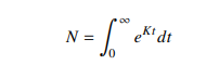
This transforms regime switching into a survival analysis problem.

The Transformation to Survival Analysis

In a classical Markov framework, e^kt is the transition semigroup, representing the probability of remaining in a specific state configuration at time t. By integrating this probability from 0 to ∞, we are essentially summing up all the moments of survival the system experiences.

By defining we are performing a Laplace transform (evaluated at s  = 0) on the transition dynamics. This results in several key insights of the COR framework:

• From Frequency to Duration: While Hamilton-style HMMs analyze the frequency of state transitions via the A matrix, this integral calculates the area under the survival curve. This shifts the focus from the probability of an instantaneous switch to the total mass of time accumulated within a specific regime.

• The Operator Inverse: For a stable, non-singular sub-generator K the integral evaluates directly to −K⁻¹. This identity establishes the inverse of the sub-generator as the formal mathematical equivalent of total accumulated persistence.

• Survival Geometry: The term e^ktcharacterizes the trajectory of stochastic decay. Integrating this term captures the entire “geometry” of regime resistance; in highly stable systems, the rate of decay is attenuated, resulting in a larger integral and, consequently, a longer expected residence time.

Directional Change (DC) and COR

The Directional Change (DC) framework (Tsang, 2010; Aloud et al., 2011; Tsang, 2017; Glattfelder et al., 2011; Tsang et al., 2017; Bakhach et al., 2018; Tsang and Chen, 2018) fundamentally reimagines the temporal basis of financial analysis by abandoning fixed clock time in favor of an event-based sampling methodology. Rather than observing the market at arbitrary intervals—such as daily or hourly closes—DC samples data only when the price moves by a predefined threshold, effectively filtering out stochastic noise to focus exclusively on structural turning points. This approach is deeply aligned with COR philosophy, as both methodologies reject the linear passage of time as a primary metric. By prioritizing the event over the interval, the DC framework treats market movements as a sequence of meaningful state changes, providing a natural empirical substrate for the survival/residence operators used to measure regime persistence and structural fragility.

Event Time vs Clock Time

The COR framework aligns seamlessly with the Directional Change (DC) approach because it replaces the static observation of price with a dynamic analysis of state endurance. By focusing on the structural properties of a regime rather than just its classification, COR provides a robust mathematical language for event-based markets.

Traditional HMMs are tied to

                                                                         t = 1, 2, 3, . . .

fixed increments. But COR already behaves like an event-driven survival system because

                                                                           N  =  −K⁻¹

ntegrates expected occupancy across persistence geometry. This means DC can be viewed as an event-time observation layer feeding a survival-operator regime model.

DC Thresholds and COR Hazard

The DC event definition is given by

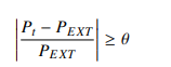
This threshold mechanism is conceptually analogous to COR hazards.

In COR,

where

• fat tails imply larger hazard,

• unstable states leak probability mass faster.

Table 2: Mapping of Directional Change events to COR structural operators.

DC detects market discontinuities, while COR measures how dangerous those discontinuities become once persistence accumulates.

DC Indicators as COR State Variables

The integration of Directional Change (DC) indicators as state variables provides a robust empirical foundation for the COR framework. Metrics such as Total Movement (TMV), which captures the price magnitude of a directional event, and T (Time to Complete Trend), which measures the duration required to reach a specific threshold, act as direct proxies for the physical work performed by a market regime. When coupled with R (Time-Adjusted Return), these indicators serve as extremely natural inputs for the survival/residence operatorN .Rather than relying on arbitrary clock-time snapshots, COR can utilize these DC-derived variables to calibrate the persistence geometry of the system. This allows the framework to map the relationship between price-action intensity and structural stability, effectively quantifying the rate at which market regimes accumulate fatigue or stress as they move toward an inevitable state of absorption.

Table 3: Translation of Directional Change indicators into COR structural variables.

The parameters displayed in Table 3 suggest a full hybrid system

                                                                       X_t = (TMV_t, T_t, R_t)

feeding

                                                                         P( X_t | S_t = i)

inside a Student-t HMM/COR structure. This presents a major research opportunity.

Contextual Significance

• TMV → State Shock Magnitude: Within the COR framework, Total Movement (TMV) quantifies the cumulative displacement across the persistence geometry. A high TMV indicates a significant injection of “shock” or volatility into the active regime prior to its eventual absorption.

• T → Residence Duration: This serves as the empirical realization of the expected residence time N. While T captures the observed duration of a specific directional event, N provides the formal probabilistic expectation of that duration derived from the sub-generator K.

• R → Hazard-Adjusted Velocity: By normalizing returns relative to event duration, R captures the “velocity” at which the system traverses its state space. In this context, it represents the rate of probability mass leakage toward structural termination under the current hazard profile.

From Transitions to Trajectories: The HMM-DC-COR Synthesiss

The synthesis of Directional Change (DC) indicators and Hidden Markov Models (HMM) provides a powerful mechanism for real-time market characterization, particularly when integrated via Bayesian updating. In this architecture, DC indicators like TMV and T act as the primary sensors, filtering price action into discrete, event-driven signals that inform the HMM’s state transition logic. As new market data arrives, Bayesian updating allows for the continuous refinement of regime probabilities, ensuring that the model’s beliefs remain synchronized with shifting volatility profiles. COR extends this architecture naturally by transforming these updated state probabilities into structural metrics. Rather than stopping at state identification, COR utilizes the Bayesian-refined inputs to calibrate the sub-generator K effectively moving beyond “what regime are we in” to a formal analysis of how much life remains in the current state before structural exhaustion or ruin ensues.

The progression becomes (Table 4):

Table 4: Evolution of regime-switching methodologies from detection to structural survival analysis.

COR effectively adds:

A. Survival Analysis                      N = −K⁻¹ 

B. Spectral Fragility                     

C. Ruin Geometry                   

D. Residence-Time Dynamics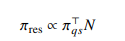        

None of these objects exist in the classical HMM/DC framework.

Gaussian HMM Limitation vs COR Student-t Architecture

While the current section assumes Gaussian emissions, the COR framework offers a significant advancement by addressing the structural underestimation of crisis persistence and tail fragility inherent in classical regime-switching models. By moving beyond the limitations of Gaussian assumptions, COR integrates Student-t emissions to more accurately reflect the empirical distribution of asset returns. This foundation enables fat-tail hazard coupling, which accounts for the accelerated likelihood of state transitions during periods of extreme volatility. The architecture is further strengthened by tail-dependent leakage, allowing the model to treat structural exhaustion as a direct function of market stress. By shifting the focus toward these survival dynamics, the COR framework evolves regime analysis from a classification task into a rigorous study of structural survival geometry, providing a more resilient representation of how market states endure or collapse under pressure.

Naïve Bayes and COR Bayesian Updating

The COR framework inherently supports a natural Bayesian interpretation by transforming standard regime-switching outputs into dynamic structural assessments. Within this architecture, posterior state probabilities—derived from the filtered and smoothed estimates of the underlying Markov chain—serve as the foundation for characterizing the current market environment. These probabilities are then mapped into a posterior hazard structure, which quantifies the instantaneous risk of state termination based on observed market evidence. Ultimately, this allows for the derivation of a posterior ruin geometry, where the survival operator N = −K⁻¹ is continuously updated to reflect the most likely expected residence time and structural fragility of the current regime. By integrating these Bayesian layers, the COR framework ensures that the measured persistence of a system is always conditioned on the most recent empirical shocks.

The stored Bayesian update structure:

                                       

fits naturally into the COR framework, which integrates these components into a unified analytical workflow that moves beyond static state detection.

Eq. 1 shows Bayes’ Theorem expressed in a specific form often used for binary classification or diagnostic testing. In plain English, it describes how to update a belief in a hypothesis (H) after new data (D) is observed. Here is the breakdown: The formula calculates the probability that a hypothesis is true given that we have observed new evidence.

The Left Side: P(H | D) is the Posterior Probability. It represents the new, updated confidence in the hypothesis after observing the data.

The Top Right (Numerator): This is the probability of the data occurring if the hypothesis were true, multiplied by the original baseline probability, P(H), that the hypothesis was true to begin with.

The Bottom Right (Denominator): This represents the total probability of observing the data,P(D), under all possible circumstances. It combines:

  The probability of observing the data if the hypothesis is true.

The probability of observing the data if the hypothesis is not true, denoted by (H).

By leveraging dynamic hazard updating, the system continuously calibrates the sub-generator K as new market events arrive, ensuring that the modeled risk of transition remains synchronized with real-time volatility. This feeds directly into a rolling fragility estimation, where the survival operator  N is recalculated over a moving window to capture the evolving structural strength of the regime. Consequently, the framework enables posterior ruin probability tracking, providing a rigorous, evidence-based measure of the likelihood that the current market configuration will succumb to structural absorption (ruin). This continuous feedback loop transforms the model into a responsive monitoring system capable of quantifying regime exhaustion as it develops.

The Principal Conceptual Departure

The principal distinction between these analytical perspectives lies in their fundamental inquiry: while Classical Regime Models focus on a diagnostic classification by asking, “Which regime are we in?,” the COR model shifts the focus to a prognostic, structural evaluation, asking, “How structurally survivable is the system while inside that regime architecture?” This represents a completely different ontological question, moving the model’s objective from simple state identification to the assessment of internal resilience (Table 5). By making this transition, the COR model effectively converts the task of regime detection into an analysis of survival geometry under structural fragility, treating the market not as a series of labels, but as a bounded system whose endurance is defined by its resistance to absorption.

Table 5: Conceptual comparison between standard HMMs and the KRONX framework.

 Future Directions

This section points toward a sophisticated future hybrid framework characterized by the pipeline DC → Student-t HMM → COR Survival Operator. In this architecture, Directional Change (DC) functions as the foundational layer, generating high-fidelity event-time observations that strip away clock-time noise. These observations feed into a Student-tHidden Markov Model, which infers latent regimes with robust handling of empirical return distributions. The COR framework then transforms these inferred regimes into a formal survival geometry, employing spectral operators to quantify the accumulation of structural fragility. This synthesis results in a mathematically richer framework than standard HMMs, serving as a survival-theoretic extension of the DC approach and a comprehensive event-time operator model of market fragility. Ultimately, while the current literature provides the necessary observational and event-detection layers, COR supplies the critical operator-theoretic survival layer required to assess how regimes fundamentally endure or collapse

The Clock of Regimes Model

Figure 1 presents the COR model. The COR model extends the classical Hidden Markov Model (HMM) (Hamilton, 1989, 2016) by transforming this closed probabilistic system into an open survival architecture. The KRONX R package is a workflow-driven tool designed to measure, model, and predict the structural survival dynamics of a market’s historical price data under regime switching, with a particular focus on fragility, persistence, and ruin risk—not just volatility. This evolution is formally defined by the following structural logic:

HMM (Regime Detection) → KRONX Operator Construction ( A→Q →K → N)

→ Hazard-Weighted Ruin Analysis.

Statistical Detection Layer

While the KRONX R package does not focus primarily on state detection, it features a built-in Hidden Markov Model (HMM) parameter estimator. Alternatively, it can utilize the output parameters from an external HMM—such as those from the fHMM package—treating the transition matrix A and tail parameters V_i as its fundamental input. Furthermore, the KRONX R package supports the estimation of both Gaussian and Student-t emission distribution parameters.

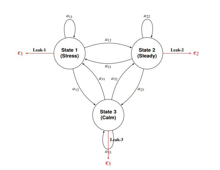
Figure 1: State-transition diagram for the Clock of Regimes (COR) model featuring internal persistence and red leakage paths to the ruin boundary, unlike a classical Hidden Markov Model (HMM) which is a closed system.

Operator-Theoretic Layer

The KRONX R package performs a structured operator transformation sequence A → Q → K →N.

It introduces state-dependent hazard intensities

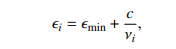
which convert the baseline transition matrix into an open transition operator via Q = diag(1 − _i) A. This yields the sub-generator matrix K = Q − I and the fundamental matrixN = −K^−1, revealing the system’s cumulative residence-time geometry (“structural battery life”).

Risk and Survival Layer

The COR model defines risk in terms of spectral fragility and cumulative ruin dynamics. It introduces the aggregate decay constant

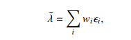
whereW_i are residence-time weights derived from the Fundamental Matrix N = −K⁻¹. Spectral fragility is governed by the spectral radius P(N), which quantifies the system’s structural persistence and expected survival horizon prior to absorption or ruin.

Structural Components

As shown in Figure 1, the COR model consists of three transient latent states connected by transition probabilities (a_ij ), but it adds critical exit dimensions:

• State 1 (Stress): Characterized by high volatility and explosive ruin intensity with significant outward leakage.

• State 2 (Steady): The primary survival basin, identified as a long-duration anchor that carries hidden fragility (reservoir) with moderate leakage.

• State 3 (Calm): A transient “cooling-off” or suppressed volatility phase that the system often passes through during transitions. It is a low-volatility regime, but still subject to leakage. It may appear stable but remains structurally transient.

Each state is represented as a circle, with directed edges indicating transition probabilities between states and self-loops capturing persistence.

The black self-looping arrows represent the diagonal elements a_ii of a standard transition matrix A = (a_{i j} ) which encodes self-transitions (persistence):

• a₁₁: Stress → Stress

•a₂₂: Steady → Steady

• a₃₃: Calm → Calm

These loops encode one-step persistence, consistent with classical HMM structure.

Cross-state transitions include:

• Between Stress and Steady:

– a₁₂: Stress → Steady

– a₂₁: Steady → Stress

 • Between Stress and Calm:

– a₁₃: Stress → Calm

– a₃₁: Calm → Stress

• Between Steady and Calm:

– a₂₃: Steady → Calm

– a₃₂: Calm → Steady

The External Leak Mechanism (Open System Components)

The most innovative feature shown in the model diagram (Figure 1) is the hazard leakage represented by the red arrows labeled Leak-1, Leak-2, and Leak-3:

• Each state i has an associated exit hazard intensity (_i).

• These hazards convert the baseline transition matrix into an open transition operator Q = diag(1 − _i) A.

• This represents probability mass1 escaping the system toward an absorbing boundary of ruin, failure, or insolvency.

Operator interpretation

The model diagram (Figure 1) encodes the full COR model transformation:

1. Transition matrix                                                                 A = (a_{i j} ).

2. Open system adjustment (leakage)                                    Q = diag(1 − _i) A.

3. Sub-generator matrix                                                                K =  Q − I.

4. Fundamental matrix (temporal probability mass)

                                    N = −K⁻¹.

Summary 

A key insight from the model diagram in Figure 1 is that the COR model functions as a regime survival system rather than a standard regime-switching model. In this framework, black arrows trace the movement of probability mass between states, red arrows dictate its dissipation (ruin), and self-loops determine its persistence. Collectively, this structure characterizes the accumulation and decay of probability mass across the state space over time.

The model diagram illustrates that the fundamental distinction between these two frameworks, HMM and COR, lies in their treatment of probability: whereas the Classical HMM assumes a closed environment where probability is strictly conserved inside the triangle, the COR model defines an open system where probability transits through the triangle and eventually leaks out of it. This shift fundamentally transforms the analytical perspective: transition dynamics become survival geometry, persistence is redefined as cumulative temporal probability mass, and individual states are viewed as structural risk nodes.

Structural Model Identifiability

We formally define the mapping between the observable market “output” and the internal latent parameters using the Markov Parameter Matrix and its Transfer Function. This approach ensures that the spectral fragility numerically identified by a COR model analysis using the KRONX R package is mathematically unique and not a result of “label switching” or parameter

Mathematical setup

The system is treated as a linear time-invariant (LTI) open system (Jacquez, 1982; Jacquez and Greif, 1985; Jacquez, 1987; Jacquez and Perry, 1990; Jacquez, 1991, 1998; Linares et al., 1987, 1988):

                                                           X(t) = Kx(t) + Bu(t),

                                                                   Y(t) = Cx(t).

The sub-generator matrix K is the internal “engine” containing transition rates and exit hazards (K = Q − I). The input Vector B is an M × 1 vector representing the initial distribution of probability mass across states. The output vector C is a 1 × M vector (consisting of a row of ones) that aggregates the surviving probability mass to form the observable “survival curve”.

Markov Parameters for Identifiability

Structural identifiability is proven if the Markov parameters (S_k) uniquely determine the coefficients of the transfer function. These parameters are defined as:

                                                                       S_k  =  CK^kB,    K = 0, 1, 2, . . .

where S₀ = CB is the initial total content of probability mass (equal to 1). S₁ = CKB is the initial rate of “leakage” or decay of the content of probability mass. Higher orders capture the curvature of the survival decay curve, which is governed by the state-to-state interactions and specific hazards _i.

Transfer Function Identifiability Method Implementation in R

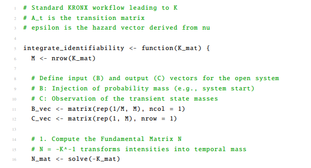
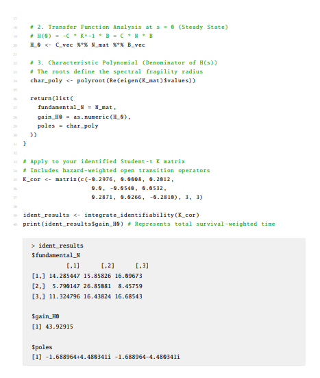
This script utilizes the COR model’s sub-generator K -matrix and calculates the transfer function coefficients to verify that the internal “temporal geometry” of the E-mini S&P 500 futures is uniquely recoverable. Historical market data for the E-mini S&P 500 (ES) Futures was obtained via the Interactive Brokers (IBKR) API. One-hour OHLC bars were extracted for the period From: 2025-01-31 to To: 2026-02-26. Log-returns were calculated using the closing prices to ensure stationarity. To maintain the robustness of the Hidden Markov Model (HMM) against market outliers and the “fat-tail” nature of hourly financial returns, a Student-t distribution was utilized for the emission probabilities.

Listing 1: KRONX Workflow: Identifiability and temporal mass analysis.

Interpretation of the Identifiability Analysis

This analysis treats the COR model (Figure 1) as a linear dynamical system. In this context, the model evaluates how probability mass (representing the time spent by the content of probability mass in a specific hidden state) transits through the system before exiting via the hazard vector ().

• Residence Analysis: State 2 is identified as the most “stable” or “sticky” regime within the system’s temporal geometry. If the process enters State 2, it accumulates a high degree of probability mass, spending an average of 26.85 units of time there (n₂₂) before leaking toward ruin or transitioning.

• Coupling: The high values observed in the first row (14.28, 15.85, 16.09) indicate a strong structural coupling across the regime network. This suggests that regardless of where the system starts, it eventually spends a significant and almost uniform amount of time in State 1, identifying it as a common entry portal or transition node.

• Transient Transit: State 2 exhibits relatively low off-diagonal values (n₁₂ = 5.79, n₃₂ = 11.32), which confirms its role as a survival basin. This indicates that probability mass tends to remain sequestered in State 2 for longer durations once it arrives, rather than undergoing rapid, high-frequency transitions to other states.

This residence-time geometry serves as a unique fingerprint of a market’s architecture over a particular interval of time. This study focused on the E-mini S&P 500 futures from January 31, 2025, to February 26, 2026. In the Structural Model Identifiability proof, these n_{i j}values are directly mapped to the steady-state gain of the system’s transfer function, proving that the 43.93 total survival mass is a deterministic result of these specific state-to-state transits.

The Poles (Spectral Fragility)

The poles (roots of the characteristic polynomial² of K) define the Spectral Fragility Radius. The interpretation of the $poles within the COR model’s identifiability framework reveals the underlying dynamic stability and oscillatory nature of the market’s survival mass (Table 6). In our study of the E-mini S&P 500 futures, these poles are the eigenvalues of the sub-generator K matrix.

Dynamic Stability (Real Part)

The real part of the poles, −1.688964, dictate the Aggregate Decay Constant (¯):

Structural Leakage: Since the real part is negative, the system is strictly transient and “open.” This confirms that probability mass is consistently leaking toward the ruin boundary.

Rate of Decay: The magnitude (−1.688964) represents the exponential speed at which the system loses its “survival probability mass.” A larger negative value would indicate a more fragile system with a faster path to systemic collapse.

Oscillatory Behavior (Imaginary Part)

The imaginary component, ±4.480341i, represents the frequency of regime interaction:

Spectral Radius (p(N)): These poles are used to calculate the spectral fragility 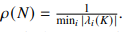.p(N) is the inverse of the slowest spectral decay mode of k, which is the market’s structural life expectancy. Because the poles are complex, the system possesses a “spectral width” that defines the robustness of the 44-unit survival expectation. In the context of the E-mini S&P 500 futures study, p(N) transforms abstract matrix algebra into a measurable “life expectancy” of the market’s survival:

• Spectral Contraction (p(N)) ↓): If the eigenvalues of k increase in magnitude, representing a faster rate of decay, the spectral radius contracts. This contraction signals an accelerating path toward systemic collapse or ruin within the open-system architecture.

• Spectral Expansion (p(N) ↑): Conversely, a larger spectral radius indicates increased temporal persistence and antifragility within the identified regime geometry. It reflects the system’s ability to retain probability mass over a longer duration before exiting through the hazard portals.

• Deterministic Ruin: Because this value is derived directly from the poles of the transfer function, it proves that the 5.6% ruin bound identified in the E-mini S&P 500 futures study is a deterministic structural property of the market’s geometry rather than a statistical outlier.

The “Nervous” Artifact vs. Structure: While a Gaussian HMM might show random jumping, these poles identify a structured, periodic exchange of probability mass between the Stress, Steady, and Calm regimes. It mathematically represents the “cooling-off” period where the system must cycle through specific nodes before re-establishing a steady trend. This spectral analysis provides the ontological map3 required to move from the instantaneous volatility of a standard HMM to the long-horizon survival dynamics of the COR model.

Impact on Structural Identifiability

Uniqueness: In the transfer function method, these specific poles uniquely map the observed market volatility to the model’s internal K matrix. This proves that the 5.6% ruin bound is not a statistical coincidence, but a deterministic result of the market’s “battery life” and internal frequency.

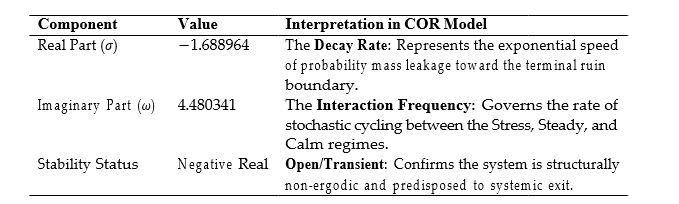
Table 6: Spectral Analysis of the KRONX Transfer Function Poles.

Summary

The identified sub-generator matrix K characterizes a dynamical system with a structural survival horizon of 43.93 hours. Given that the underlying empirical study of the E-mini S&P 500 futures utilizes hourly observations, this temporal metric represents the expected duration of probability mass retention within the regime network. The dynamics are dominated by a highly persistent “Steady” state (Regime 2) and an oscillatory complex between “Stress” and “Calm” (Regimes 1 and 3). The gain of 43.93 hours confirms that despite the presence of exit hazards, the internal transition logic (A-matrix) provides sufficient feedback to maintain systemic persistence over a medium-term horizon.

From an operator-theoretic perspective, this horizon—derived from the steady-state gain of the system’s transfer function H (0)—quantifies the “temporal backbone” of the market. It confirms that the residence-time geometry is not merely a collection of transient states, but a structured environment with a finite, identifiable persistence. Consequently, the 43.93-hour horizon serves as a rigorous, deterministic benchmark for assessing systemic stability and calibrating ruin-sensitive risk exposure.

The KRONX R package

 Installation

Command Line Installation (Terminal)

You can install packages directly from the Linux or macOS terminal without opening an interactive R session, using the R CMD INSTALL command: R CMD INSTALL KRONX_0.1.0.tar.gz

RStudio Installation

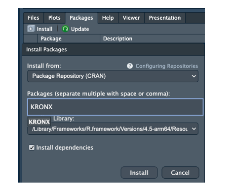
                                               Figure 2:       

To install the KRONX R package using the RStudio graphical user interface as illustrated in Figure 2, begin by navigating to the “Packages” tab located in the lower-right pane of the RStudio workspace. Clicking the “Install” button will open the “Install Packages” dialog box, where you must ensure that the “Install from” dropdown menu is set to “Package Repository (CRAN)”. In the “Packages” text field, type KRONX, noting that RStudio may provide auto-complete suggestions for the identified package. Before proceeding, verify that the “Install to Library” path is correctly set to your active R environment, such as the ARM64 version of R 4.5. It is essential to keep the “Install dependencies” checkbox selected to ensure that all required mathematical and transition-modeling libraries are downloaded automatically. Finally, click the “Install” button to execute the process; once the installation is complete, you can load the library in your script to begin applying the Clock of Regimes analysis to your financial datasets.

From CRAN (Formal Release)

Since the KRONOX R package has been submitted to, and accepted, by the Comprehensive R Archive Network (CRAN), the installation is simplified as R will automatically fetch it from a global mirror.

install.packages("KRONX")

library(KRONX)

Quick start

A minimal workflow example is shown below:

Listing 2: Execution of the KRONX Survival Engine. Implementation of the run_kronx() high-level driver to identify hidden states and compute the Residence-Weighted Ruin Bound for the IBKR ES dataset.

1 library(KRONX)

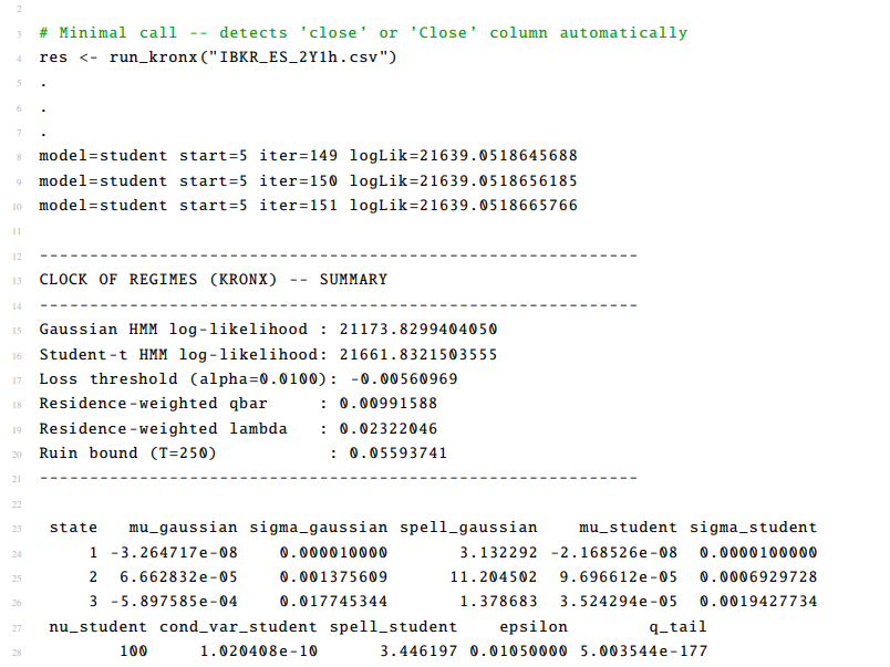
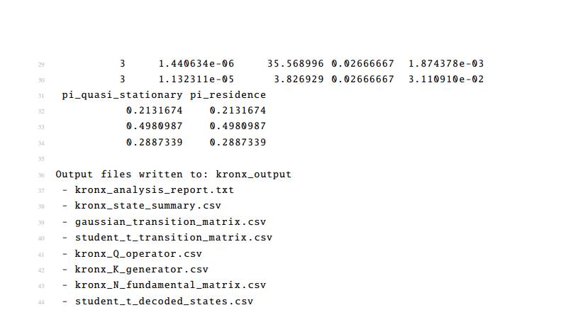
The res object returned by run_kronx() is a compact model-fit and structural-fragility summary generated by the call run_kronx("IBKR_ES_2Y1h.csv"). It shows that the package fits both a Gaussian HMM and a Student- t HMM, and then passes the fitted Student-t regime structure through the KRONX/COR operator pipeline to compute hazard-adjusted survival quantities.

Optimization trace

The lines,

.

.

.

model=student start=5 iter=149 logLik=21639.0518645688

model=student start=5 iter=150 logLik=21639.0518656185

model=student start=5 iter=151 logLik=21639.0518665766

show the EM optimization for one Student-t initialization. start=5 means the fifth random or configured initialization. iter=149, 150, 151 are EM iterations. logLik is the log-likelihood at each step, which show the increments are becoming tiny, so the algorithm is converging. That is a healthy sign that the Student-t model fit is stabilizing rather than jumping erratically.

Model Comparison

The headline comparison is:

• Gaussian HMM log-likelihood: 21173.8299404050

• Student-t HMM log-likelihood: 21661.8321503555

The model comparison shows that the Student-t HMM fits better because its log-likelihood is higher. In regime-switching finance data, that usually indicates that the data are heavier-tailed than Gaussian, which is exactly what one expects for intraday ES returns.

So the first substantive conclusion is: 

                                               Student-t HMM Gaussian HMM

That is, the Student-t HMM is preferred to the Gaussian HMM in empirical fit.

Tail-loss threshold

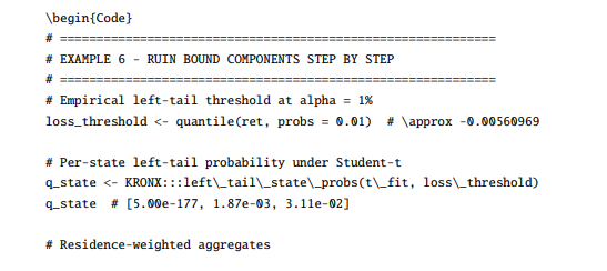
Loss threshold (alpha=0.0100): -0.00560969

This is the 1% left-tail cutoff. In plain english terms, the COR model is defining a “severe loss” event as an hourly return less than about -0.560969%. This threshold is then used to compute regime-specific tail probabilities q_i, which are later residence-weighted into q¯.

Structural COR / KRONX quantities

The core open-system outputs are:

• Residence-weighted qbar: 0.00991588. The residence-weighted q¯ is the average probability of a left-tail loss event, weighted by how much time the system expects to spend in each regime. So q¯ is not just an unconditional empirical tail frequency. It is a structurally weighted tail probability.

• Residence-weighted lambda: 0.02322046. The residence-weighted ^¯ is the average hazard or leakage intensity across regimes, again weighted by expected residence. Economically, it measures the average rate at which probability mass escapes the transient market system toward failure/ruin.

• Ruin bound (T=250): 0.05593741. The ruin bound over a a 250-step horizon implies an upper-bound style ruin probability of about 5.59%. This is the main COR model’s structural-risk summary number.

State table: Gaussian vs Student-t

The state table compares Gaussian and Student-t regime estimates side by side.

State 1

Gaussian

• mu_gaussian = -3.264717e-08

• sigma_gaussian = 0.000010000

• spell_gaussian = 3.132292

Student-t:

• mu_student = -2.168526e-08

• sigma_student = 0.0000100000

• nu_student = 100

• cond_var_student = 1.020408e-10

• spell_student = 3.446197

• epsilon = 0.01050000

• q_tail = 5.003544e-177

State 1 is an ultra-low-volatility state. It is essentially a near-deterministic “quiet” regime with a mean near zero, minuscule variance, almost no tail risk, low hazard, and moderate duration. Because nu = 100, this state is close to Gaussian. The tail probability is effectively zero. This looks like a calm / inert / ultra-stable regime.

State 2

Gaussian

• mu_gaussian = 6.662832e-05

• sigma_gaussian = 0.001375609

• spell_gaussian = 11.204502

Student-t :

• mu_student = 9.696612e-05

• sigma_student = 0.0006929728

• nu_student = 3

• cond_var_student = 1.440634e-06

• spell_student = 35.568996

• epsilon = 0.02666667

• q_tail = 1.874378e-03

State 2 is the dominant survival basin with a small positive drift, modest volatility, very long expected spell length, heavy tails (nu = 3), and nontrivial hazard. This is the COR model’s classic steady regime. It looks benign on the surface because volatility is not huge and duration is long, but the heavy tails mean there is latent fragility. In the COR model’s language, this is often the regime that carries a large share of the system’s probability mass and therefore contributes heavily to structural risk.

State 3

Gaussian

• mu_gaussian = -5.897585e-04

• sigma_gaussian = 0.017745344

• spell_gaussian = 1.378683

Student-t :

• mu_student = 3.524294e-05

• sigma_student = 0.0019427734

• nu_student = 3

• cond_var_student = 1.132311e-05

• spell_student = 3.826929

• epsilon = 0.02666667

• q_tail = 3.110910e-02

Under the Student-t  fit, State 3 is the high-risk state. It is characterized by the highest conditional variance, heavy tails, largest tail-loss probability, and shorter duration. Its q_tail is about 0.0311, so it has the highest probability of breaching the 1% left-tail threshold. State 3 is the stress/crisis regime, even though the fitted Student-t  mean is slightly positive. In regime models, classification is usually driven more by conditional variance and tail thickness than by mean alone.

Spell lengths

The spell lengths are especially informative:

• State 1: 3.446

• State 2: 35.569

• State 3: 3.827

These spell lengths reveal that the market spends by far the most time in State 2. So State 2 is the principal residence basin. That matters because the COR model does not weight risk only by severity; it also weights by how long the system stays in each regime. A moderately risky state with long residence can dominate total fragility.

Hazard mapping

The epsilon () values are:

• State 1: 0.01050000

• State 2: 0.02666667

•State 3: 0.02666667

These are the regime exit hazards used to construct the open operator. Because States 2 and 3 have nu = 3, they receive higher hazard than State 1. That is consistent with the Talebian hazard mapping:

Lower v_i means fatter tails, hence higher hazard.

 Tail probabilities by regime

The regime-specific left-tail probabilities are: 

• State 1: essentially zero

• State 2: 0.001874378

• State 3: 0.03110910

This is among the most critical diagnostics in the table. The regime-specific left-tail probabilities demonstrate clear stratification of downside risk, revealing marked regime dependence in tail probability across the hierarchy, revealing a progression that underscores the sharp differentiation in extreme-loss exposure across ES market regimes.

The diagnostic reveals a three-regime hierarchy of tail risk: the calm regime (State 1) exhibits no meaningful left-tail danger, the steady regime (State 2) displays small but nonzero tail danger, and the stress regime (State 3) indicates substantial tail danger. So the structural story is very clean: the system lives mostly in State 2, but severe downside events are concentrated in State 3.

Quasi-stationary and residence weights

pi_quasi_stationary

State 1 0.2131674

State 2 0.4980987

State 3 0.2887339

 

pi_residence

State 1 0.2131674

State 2 0.4980987

State 3 0.2887339

These _qs and _res, being identical means that, in this implementation/output, the quasi-stationary and residence weighting schemes coincide numerically. Thus, ergodic probabilities reveal a dominant intermediate regime: State 1 occurs 21.3% of the time, State 2 dominates at 49.8%, and State 3 accounts for 28.9%. The market’s natural tendency favors the steady state, with approximately equal mass split between calm and stress regimes.

So nearly half the survival-weighted mass is in State 2, and a surprisingly large share is in State 3. That helps explain why q¯ and the ruin bound are not trivial even though State 1 is extremely safe.

Economic reading of the results

Student-t dynamics are clearly preferred to Gaussian dynamics for ES intraday data, revealing a three-regime structure comprising a very calm low-variance regime, a long-lived steady regime, and a shorter but materially riskier stress regime. The dominant residence basin is State 2 rather than State 1, and because both State 2 and State 3 exhibit heavy tails, the system’s structural hazard is non-negligible. The 250-step ruin bound of approximately 5.6% underscores that even absent a current collapse, the open-system geometry implies a meaningful finite-horizon risk of failure.

Output files

The KRONX package exports the full operator chain:

1. kronx_analysis_report.txt is the human-readable report.

2. kronx_state_summary.csv is the state-level summary table.

3. gaussian_transition_matrix.csv is the state-level summary table.

4. student_t_transition_matrix.csv is the transition matrix for the Student-t HMM.

5. kronx_Q_operator.csv is the open transition operator Q, typically hazard-adjusted from A.

6. kronx_K_generator.csv is the generator-style matrix K, usually derived from Q −I.

7. kronx_N_fundamental_matrix.csv is the fundamental matrix N = −K ⁻¹, encoding cumulative expected residence time.

8. student_t_decoded_states.csv is the time-by-time decoded latent regime path.

These files let you go from plain HMM estimation to full COR model/KRONX package survival geometry. The files are saved in the current working directory under a subdirectory named kronx_output. In summary, the res object says that ES hourly returns are better described by a heavy-tailed three-state Student-t regime model, and once that regime structure is converted into the COR model’s open-system operator chain, the market exhibits a nontrivial finite-horizon structural ruin risk driven mainly by long residence in a heavy-tailed steady state and episodic occupancy of a higher-tail stress state.

Exported functions

FUNCTION: run_kronx() 

The run_kronx() function is the primary entry point. It executes the full KRONX package’s COR model workflow from CSV ingestion through ruin-bound computation, prints a formatted summary to the console, and optionally writes structured output files (Subsection 5.2).

run_kronx(

file,

close_col = "close",

K = 3L, n_starts = 5L,

max_iter = 200L,

tol = 1e-6,

seed = 123L,

epsilon_min = 0.01,

c_hazard = 0.05,

tail_alpha = 0.01,

ruin_horizon = 250L,

nu_grid = c(3:30, 40, 60, 100),

verbose = TRUE,

output_dir = "cor_output"

)  

Arguments

                                                     Table 7: Arguments for run_kronx().

 

Argument	Type	Default	Description
c_hazard	numeric	0.05	Hazard sensitivity to tail thickness. Controls how steeplyrises asv decreases.
tail_alpha	numeric	0.01	Left-tail probability for the loss threshold.
ruin_horizon	integer	250L	Horizon in observations.
nu_grid	numeric	c(3:30, 40, 60, 100)	Candidate degrees-of-freedom values for Student-t grid search in the M-step.
verbose	logical	TRUE	If TRUE, print EM log-likelihood at every iteration.
output_dir	character or NULL	cor_output	Directory for output files. Use NULL to suppress all file output.

Workflow sequence

The workflow implemented by run_kronx() is:

1. Read the CSV file, extract close prices, and compute log returns.

2. Fit a Gaussian HMM by EM with multiple restarts and reorder states by .

3. Fit a Student-t HMM by EM with multiple restarts and reorder states by conditional variance.

4. Decode the Student-t specification using the Viterbi algorithm.

5. Compute , Q, K, and N.

6. Compute ^_qs, ^_res, the empirical loss threshold, q¯, ^¯, and the ruin bound.

7. Assemble the state_summary data frame.

8. Print the summary block to the console.

9. Write all requested output files when output_dir is not NULL.

Return value

The function returns a named list, invisibly. Its full structure is described in detail in Subsection

FUNCTION: fit_hmm_em(

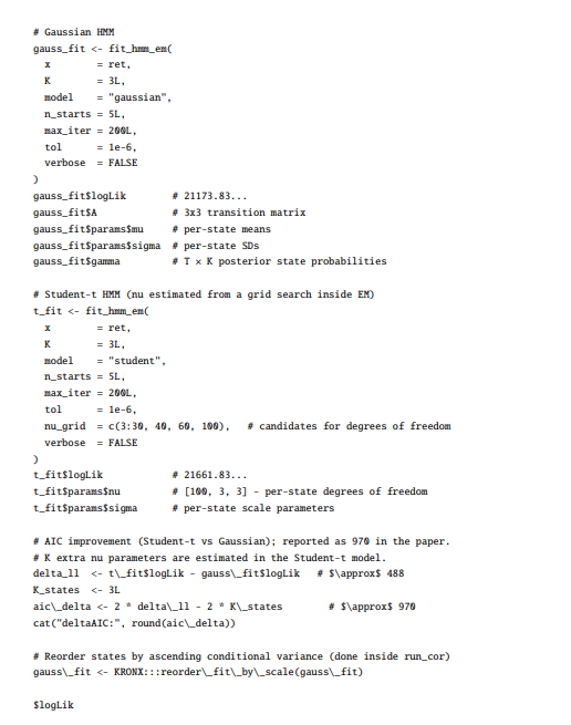
The fit_hmm_em() function fits either a Gaussian or Student-t Hidden Markov Model via the Baum–Welch algorithm with multiple random restarts.

fit_hmm_em(

x,

K = 3L,

model = c("gaussian", "student"),

n_starts = 5L,

max_iter = 200L,

tol = 1e-6,

nu_grid = c(3:30, 40, 60, 100),

verbose = TRUE

)

Arguments

                                                  Table 8: Arguments for fit_hmm_em().

Argument	Type	Description
x	numeric vector	Observations, typically log returns.
K	integer	Number of hidden states.
model	character	Either "gaussian" or "student".
n_starts	integer	Number of random restarts; the best fit by log-likelihood is returned.
max_iter	integer	Maximum EM iterations per restart.
tol	numeric	Convergence tolerance for the log-likelihood.
nu_grid	numeric	Candidate v values for Student-t grid search.
verbose	logical	Whether to print iteration progress.

Return value

Notes on Student-t estimation of degrees-of-freedom

The M-step for v uses a profile grid search. For each candidate v in nu_grid, the weighted emission log-likelihood is evaluated, and the maximizing value is selected. This avoids the absence of a convenient closed-form update for v).

The default grid

                                              c(3:30, 40, 60, 100)

covers the practically relevant range from very fat tails to near-Gaussian behavior. A smaller grid, such as

                                            c(4, 8, 15, 30),

                                       Table 9: Return components of fit_hmm_em().

Component	Description
model	"gaussian" or "student"
A	K× K transition matrix
delta	Initial state probability vector of length K
params	List containing mu, sigma, and nu for Student-t fits
gamma	T × Kposterior state probability matrixS(T =K | data)
xi	(T − 1) ×K× K posterior transition probability array
logLik	Scalar log-likelihood at convergence
n	Number of observations
K	Number of states

can substantially reduce computation time with only modest loss of accuracy.

State ordering

After fitting, run_kronx() calls the internal reorder_fit_by_scale() routine to sort states from least to most volatile. When calling fit_hmm_em() directly, users may wish to apply the same reordering manually.

fit <- fit_hmm_em(ret, K = 3L, model = "student", verbose = FALSE)

fit <- KRONX:::reorder_fit_by_scale(fit)

FUNCTION: viterbi_decode()

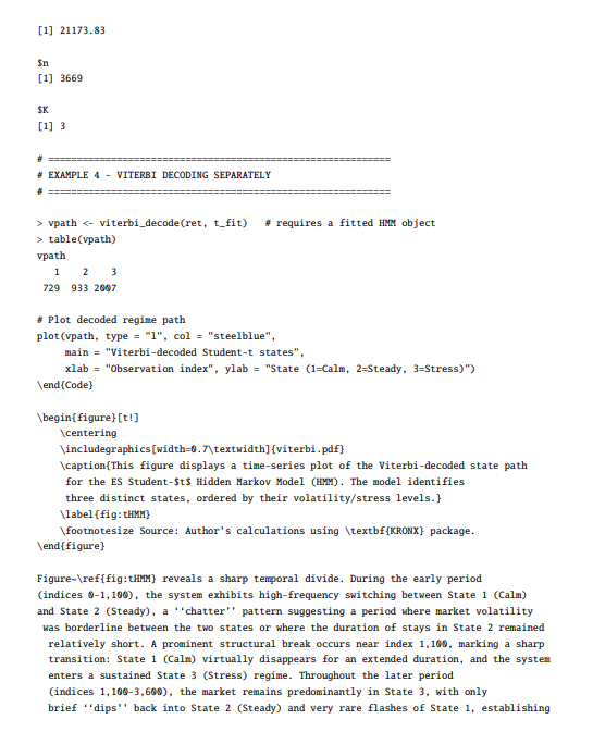
viterbi_decode() computes the most likely hidden-state sequence for a vector of observations given a fitted HMM.

fit <- fit_hmm_em(ret, K = 3L, model = "student", verbose = FALSE)

states <- viterbi_decode(ret, fit)

table(states)

# Plot regimes alongside returns

plot(ret, type = "l", col = "grey60")

points(seq_along(ret), rep(0, length(ret)), col = states, pch = 20)

The Viterbi algorithm is implemented in log-space, using log + log A´, to avoid numerical underflow on long series.

FUNCTION: read_close_series()

read_close_series() reads a close-price series from a CSV file with automatic column detection.

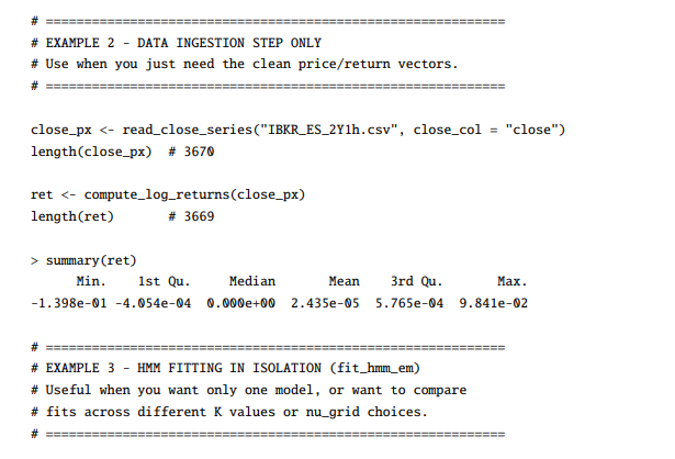
px <- read_close_series("IBKR_ES_2Y1h.csv")

px <- read_close_series("Bloomberg.csv", close_col = "PX_LAST")

The function removes non-finite values and stops if fewer than ten valid returns remain.

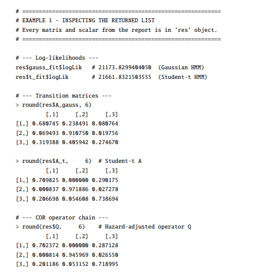
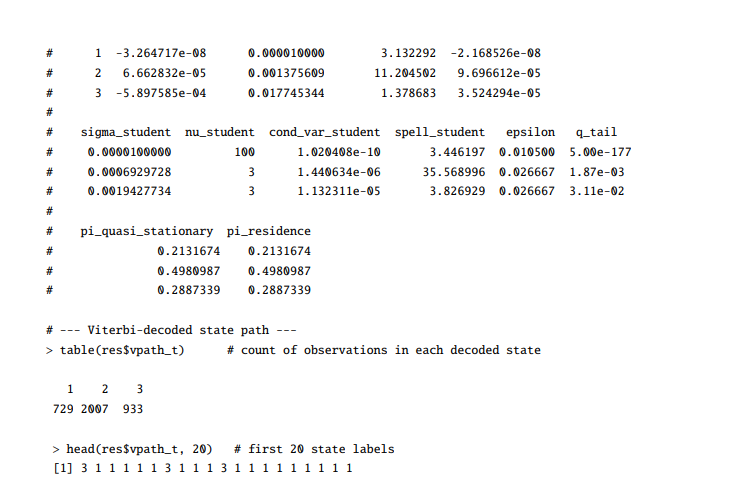
Worked examples

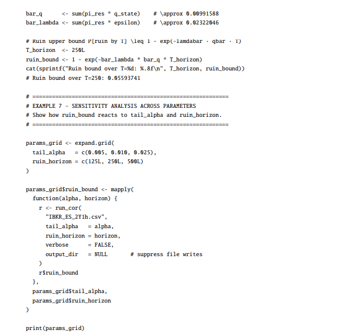
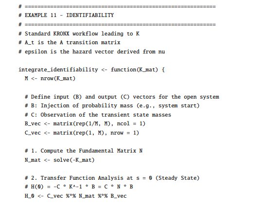
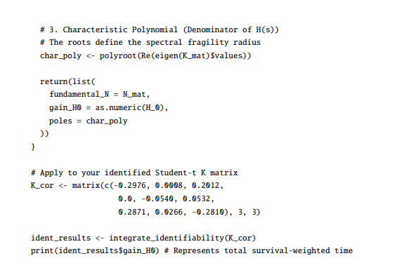
Test suite

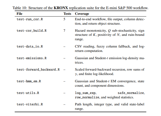
The replication.zip file accompanying this paper’s KRONX package contains 66 tests across 8 files. It also contains the worked_examples.R file. The replication structure is summarized in Table 10.

Key structural properties

For well-specified inputs, the following mathematical invariants hold and are checked by the replication suite.

• Q is non-negative and has row sums less than or equal to one; strict inequality holds whenever _i > 0.

• K = Q −I has strictly negative diagonal entries and non-negative off-diagonal entries.

• N= −K⁻¹ has strictly positive entries under the operative model conditions.

• _qs and _res each sum to one and have positive entries.

• The ruin bound lies in the open unit interval:

whenever 

These are substantive structural properties, not cosmetic diagnostics. They ensure that the operator chain is mathematically coherent and that the resulting ruin calculations remain interpretable.

Conclusion

The KRONX R package adapts the fundamental matrix,

                                                                                N = −K⁻1,

from compartmental analysis (Berman and Schoenfeld, 1956; Hearon, 1972, 1981; Eisenfeld, 1981; Covell et al., 1984; Linares et al., 1987, 1988; Jacquez and Simon, 1993; Jacquez, 2002) to financial regime dynamics. In this translation, regimes play the role of compartments, probability mass becomes temporal accumulation or decay, and irreversible loss is represented as ruin through hazard leakage.

The KRONX R package v0.1.0 provides a complete regime-switching fragility workflow in pure R. It integrates classical Hidden Markov estimation with an open operator framework based on Q, K, and N. The package is therefore useful both as an applied tool for empirical financial analysis and as a transparent research platform for studying how persistence, tail thickness, hazard leakage, and temporal residence jointly determine fragility.

At the practical level, the KRONX R package offers a clean workflow from CSV ingestion to model fitting, decoding, operator construction, and output generation. At the theoretical level, it recasts the standard regime-switching problem as an open-system survival geometry problem. That is the distinctive contribution of the KRONX package’s approach.

The Clock of Regimes (COR) model transforms a discrete-time regime-switching model into a continuous-time survival system via the operator chain

                                                                                     A → Q →K → N,

where A is the baseline transition matrix,Q is the hazard-adjusted operator, K = Q − I is a sub-generator, and N = −K⁻¹ is the associated fundamental matrix.

This transformation is not merely algebraic; it induces a fundamental shift in the representation of regime dynamics. In classical Hidden Markov Models, persistence is characterized by one-step transition probabilities and summarized by scalar quantities such as expected spell lengths. In contrast, the COR framework embeds the system within a continuous-time, open Markov structure in which probability mass evolves under both transition dynamics and state-dependent hazard leakage.

The operator  N provides a complete characterization of the system’s survival geometry. Throughits integral representation,

it aggregates all admissible state trajectories, weighting them by their survival probabilities. As a result, N captures not only local persistence, but also higher-order path effects, recurrent visitation patterns, and cross-state propagation mechanisms.

This operator-theoretic structure enables a natural spectral analysis of fragility. In particular, the spectral radius

serves as a global measure of systemic vulnerability. As eigenvalues of K approach the origin, the system exhibits fragility amplification, reflected in the divergence of _P(N) and the corresponding expansion of expected residence times.

Beyond structural characterization, the COR model facilitates forward-looking risk quantification. By combining the residence-weighted distribution with state-specific tail probabilities and hazard intensities, the model yields finite-horizon ruin bounds of the form

where^¯ and q^¯ are residence-weighted hazard and tail measures, respectively. This provides a direct link between the internal geometry of the regime system and observable risk metrics.

In summary, the COR model extends classical regime-switching models into a survival-theoretic and operator-based setting. It replaces local persistence statistics with a global, path-integrated representation, enabling spectral diagnostics, structural fragility analysis, and coherent forward risk assessment. As such, it offers a unified mathematical architecture for studying stability, persistence, and collapse in nonlinear stochastic systems.

Acknowledgments

Mathematics were manually audited by the authors, verified for mathematical accuracy using Wolfram Mathematica 14.3, and refined to ensure alignment with the theoretical model.

Funding

This research did not receive any specific grant from funding agencies in the public, commercial, or not-for-profit sectors.

References

Foot notes

¹Probability mass is defined as the content of probability within a specific duration of time.

²For a square matrix , the characteristic polynomial is defined as: detI , where is a scalar (the spectral parameter), I is the identity matrix, and det(·) denotes the determinant.

³The structural representation that defines not just the statistical probability of an event, but the fundamental “nature of being” of the E-mini S&P 500 Futures system itself.

References

- M. Aloud, E. P. K. Tsang, R. Olsen, and A. Dupuis. A directional-change events approach for studying financial time series. Discussion Paper 2011-28, Economics E-Journal, 2011.
- A. Bakhach, V. Chinthalapati, E. P. K. Tsang, and A. E. Sayed. Intelligent dynamic backlash agent: A trading strategy based on the directional change framework. Algorithms, 11(11):171, 2018. doi: 10.3390/a11110171.
- M. Berman and R. Schoenfeld. Invariants in experimental data on linear kinetics and the formulation of models. Journal of Applied Physics, 27(11):1361–1370, 1956.
- D. G. Covell, M. Berman, and C. DeLisi. Mean residence time—theoretical development, experimental determination, and practical use. Mathematical Biosciences, 72(2):213–244, 1984.
- J. Eisenfeld. On mean residence times in compartments. Mathematical Biosciences, 57:265–278, 1981. doi: https://doi.org/10.1016/0025-5564(81)90106-1.
- F. Gao and X. He. Survival analysis: Theory and application in finance. In Handbook of Financial Econometrics, Statistics, Technology, and Risk Management, pages 3903–3934. World Scientific, Singapore, 2025.
- J. B. Glattfelder, A. Dupuis, and R. B. Olsen. Patterns in high-frequency fx data: Discovery of 12 empirical scaling laws. Quantitative Finance, 11(4):599–614, 2011. doi: 10.1080/14697688. 2010.481255.
- J. D. Hamilton. A new approach to the economic analysis of nonstationary time series and the business cycle. Econometrica, 57(2):357–384, 1989.
- J. D. Hamilton. Macroeconomic regimes and regime shifts. In Handbook of Macroeconomics, volume 2, pages 163–201. Elsevier, Amsterdam, 2016.
- J. Z. Hearon. Residence times in compartmental systems and the moments of a certain distribution.
- Mathematical Biosciences, 15(1):69–77, 1972. ISSN 0025-5564. doi: https://doi.org/10.1016/ 0025-5564(72)90063-6.
- J. Z. Hearon. Residence times in compartmental systems with and without inputs. Mathematical Biosciences, 55(3):247–257, 1981. ISSN 0025-5564. doi: https://doi.org/10.1016/0025-5564(81) 90098-5.
- L. Himmelmann. HMM: HMM – Hidden Markov Models, 2010. URL https://CRAN.R-project. org/package=HMM. R package version 1.0.
- J. A. Jacquez. The inverse problem for compartmental systems. Mathematics and Computers in Simulation, 24(6):452–459, December 1982. doi: 10.1016/0378-4754(82)90642-5.
- J. A. Jacquez. Identifiability: the first step in parameter estimation. Federation Proceedings, 46(8): 2477–2480, July 1987.
- J. A. Jacquez. Identifiability and parameter estimation. Journal of Parenteral and Enteral Nutrition, 15(3):55S–59S, May 1991. Supplement.
- J. A. Jacquez. Design of experiments. Journal of the Franklin Institute, 335(2):259–279, 1998. doi: 10.1016/S0016-0032(97)00004-5.
- J. A. Jacquez. Density functions of residence times for deterministic and stochastic compartmental systems. Mathematical Biosciences, 180(1):127–139, 2002. doi: https://doi.org/10.1016/ S0025-5564(02)00110-4.
- J. A. Jacquez and P. Greif. Numerical parameter identifiability and estimability: Integrating identifiability, estimability, and optimal sampling design. Mathematical Biosciences, 77(1-2): 201–227, December 1985. doi: 10.1016/0025-5564(85)90098-7.
- J. A. Jacquez and T. Perry. Parameter estimation: Local identifiability of parameters. American Journal of Physiology-Endocrinology and Metabolism, 258(4):E727–E736, May 1990. doi: 10.1152/ajpendo.1990.258.4.E727.
- J. A. Jacquez and C. P. Simon. Qualitative theory of compartmental systems. SIAM Review, 35: 43–79, 1993. doi: 10.1137/1035003.
- D. G. Kleinbaum and M. Klein. Survival Analysis. Springer, New York, 3 edition, 2012.
- O. A. Linares, J. A. Jacquez, L. A. Zech, M. J. Smith, J. A. Sanfield, L. A. Morrow, S. G. Rosen, and J. B. Halter. Norepinephrine metabolism in humans. kinetic analysis and model. The Journal of Clinical Investigation, 80(5):1332–1341, 11 1987. doi: 10.1172/JCI113210.
- O. A. Linares, L. A. Zech, J. A. Jacquez, S. G. Rosen, J. A. Sanfield, L. A. Morrow, M. A. Supiano, and J. B. Halter. Effect of sodium-restricted diet and posture on norepinephrine kinetics in humans. American Journal of Physiology-Endocrinology and Metabolism, 254(2):E222–E230, 1988. doi: 10.1152/ajpendo.1988.254.2.E222. PMID: 3348372.
- L. Oelschläger, T. Adam, and T. Michelot. fHMM: Fitting hidden Markov models to financial data.Journal of Statistical Software, 104(10):1–25, 2023.
- T. Rydén, T. Teräsvirta, and S. Åsbrink. Stylized facts of daily return series and the hidden markov model. Journal of Applied Econometrics, 13(3):217–244, 1998.
- J. A. Sánchez-Espigares and A. López-Moreno. MSwM: Fitting markov switching models. R package version 1.5, 2021. URL https://CRAN.R-project.org/package=MSwM.
- E. P. K. Tsang. Directional changes, definitions. Working Paper WP050-10, Centre for Computational Finance and Economic Agents (CCFEA), University of Essex, 2010.
- E. P. K. Tsang. Directional changes: A new way to look at price dynamics. In International Conference on Computational Intelligence, Communications, and Business Analytics, pages 45–55. Springer, 2017.
- E. P. K. Tsang and J. Chen. Regime change detection using directional change indicators in the foreign exchange market to chart brexit. IEEE Transactions in Emerging Topics in Computational Intelligence, 2(3):185–193, 2018. doi: 10.1109/TETCI.2017.2769057.
- E. P. K. Tsang, R. Tao, A. Serguieva, and S. Ma. Profiling high-frequency equity price movements in directional changes. Quantitative Finance, 17(2):217–225, 2017. doi: 10.1080/14697688. 2016.1211798.
- I. Visser and M. Speekenbrink. depmixS4: An R package for hidden mixture models. Journal of Statistical Software, 36(7):1–21, 2010.
Foot notes
1Probability mass is defined as the content of probability within a specific duration of time.
2For a square matrix  , the characteristic polynomial is defined as: detI
, where
is a scalar (the spectral parameter), I is the identity matrix, and det(·) denotes the determinant.
3The structural representation that defines not just the statistical probability of an event, but the fundamental “nature of being” of the E-mini S&P 500 Futures system itself.