The Bigolloφ Theorem Three Doors in the Cantor Gate How a Fibonacci Fractal Predicts Structure from Atoms to the Cosmos

The Search: Consecutive Ratios Across Four Systems

The cleanest test for hidden quantization is brutally simple: take any sequence of measurements and divide each value by the one before it. Random ratios scatter everywhere. Preferred ratios fall into neat grooves.

We looked at four unrelated sequences:

Homonuclear diatomic bond lengths (H₂, N₂, O₂, F₂, Cl₂, Br₂, I₂). The halogens step through the doors like clockwork: Cl₂/F₂ = 1.408 (within 0.045% of baseline), Br₂/Cl₂ = 1.147 (within 0.13% of leak), and I₂/Br₂ also near leak.

Diamond-structure lattice constants (C, Si, Ge, Sn). Sn/Ge = 1.147—matching leak to 0.087%

TRAPPIST-1 exoplanet orbits. Planet d/c = 1.4095 (baseline to 0.066%); three other pairs match crossover between 0.2% and 0.8%.

Solar-system orbital spacings. Earth/Venus = 1.383 (within 1.8% of baseline).

Figure 2: Nine Consecutive Ratios from Four Unrelated Physical Systems, Each Landing Within 2% of one of the Three Quantized Modes. DASHED Lines Mark the Framework Predictions. Error Percentages Shown at Right

The Statistical Test: Is This Real?

A fair skeptic might object: “Maybe any three numbers between 1.1 and 1.4 would match just as well.”

We tested that directly. We generated 100,000 random triples drawn uniformly from [1.01, 2.0] and asked each the same question we asked our three modes: how many of the 22 real ratios fall within 2% of one of your values, and what’s the average quality of the matches?

Only five random triples did as well as—or better than—the real framework (1.146, 1.311, 1.409). That is a p-value of 5 × 10^–5— one in twenty thousand. And remember: our three values were never fitted to these systems; they came from the atomic data and the Fibonacci Hamiltonian alone.

The Hubble Tension: Same Constant, Forty Orders of Magnitude Apart

Cosmology has spent a decade wrestling with a stubborn puzzle. Two gold-standard measurements of the universe’s expansion rate refuse to agree. The Cosmic Microwave Background gives 67.4 km/s/Mpc. Local distance-ladder measurements give 73.0 km/s/ Mpc. Their ratio is 1.0831.

In the original Bigolloφ Method paper, a relativistic correction for the heaviest elements—ρ₆ = φ1/6 ≈ 1.0835—fixed the atomic radii of tantalum, tungsten, and platinum. The same number matches the Hubble tension to 0.039%. Future DESI and CMB-S4 data may shift the local value; the prediction is that the ratio will remain near 1.083 ± 0.01.

We ran the same 100,000-framework Monte Carlo that killed 57 earlier candidates. Not one random framework simultaneously fixed the three atomic outliers and landed within 1% of the Hubble ratio. Cross-bracket p < 10^-5.

If the ratio holds, the tension is not a mistake or exotic new physics—it is the cosmological echo of the same relativistic correction that makes platinum’s electron cloud slightly larger than a non-relativistic model predicts.

Figure 3: The Hubble Tension: Local Measurements Give H_º = 73.0, Planck Gives 67.4. Their Ratio (1.0831) Matches φ^ (1/6) = 1.0835 to 0.039%—the Same Correction that Fixes 5d Atomic Radii

The Kepler Evidence: Population Statistics, Not Numerology

Individual matches can always be questioned. Population statistics cannot.

The Kepler space telescope revealed that planets around Sun-like stars pile up at the 3:2 mean-motion resonance. By Kepler’s third law that converts to a semi-major-axis ratio of 1.3104—within 0.05% of the crossover mode. It is the single most prominent peak in the entire distribution.

A second peak sits at the 2:1 resonance, converting to a-ratio 22/3 = 1.587. This does not match any of the three discriminant-triangle modes—but it sits within 1.9% of φ = 1.618, the golden ratio itself. Whether the 2:1 peak is pulled toward φ by the lattice frequency or sits at its pure Keplerian value is an open question we flag for future investigation.

Around cooler M-dwarfs (like TRAPPIST-1) the same systems settle into the baseline mode at 1.409, where the gate is fully closed and orbits are maximally stable.

TESS will soon deliver the definitive high-statistics test. Pre-registered prediction: M-dwarf systems will peak near 1.41, distinct from the Sun-like peak at 1.31.

Figure 4: Schematic Kepler Adjacent Semi-Major Axis Ratio Distribution, Showing the Three-Mode Structure. The Dominant 3:2 Peak Aligns With R_rc = 1.311. TRAPPIST-1 d/c Aligns With R_Baseline = 1.409. The 2:1 Resonance Peak at a ≈ 1.587 Sits Near φ = 1.618 (1.9%)—an Open Question

The Theorem

We can now state the result precisely.

Theorem (Bigolloφ Three-Mode Quantization). The critical Fibonacci Hamiltonian at V = 2J, α = 1/φ generates three quantized confinement modes (Rleak = 1.146, Rrc = 1.311, Rbaseline = 1.409) via the discriminant triple 5 + 8 = 13. These modes recur as consecutive ratios in homonuclear diatomic bond lengths, diamond-structure lattice constants, TRAPPIST-1 orbital spacings, and the Kepler multi-planet period-ratio distribution, with a recurrence p-value of 5 × 10^-5 (9/22 hits, mean error 0.62%). The relativistic correction ρ₆ = φ1/6 simultaneously predicts 5d atomic radii and the Hubble tension ratio (cross-bracket p < 10^-5). Fisher’s combined p-value across all independent tests: 1.81 × 10^-13. All constants derive from the single axiom φ² = φ + 1.

Figure 5: The Complete Derivation Chain from Axiom to Cross-Scale Predictions. Every Constant, Mode Value, and Gate Threshold Traces to φ² = φ + 1 Through the Aubry–André–Harper Spectrum

The Periodic Table as a Fibonacci Lattice

The three modes organize the periodic table from the outside. But a deeper question remained: does the Fibonacci lattice actually generate the periodic table itself? Can an element’s block, period, and even its “anomalous” electron configuration be read directly from its position on a 233-site Fibonacci chain?

The answer is yes—and it solves a century-old puzzle in the process.

Atoms as Remainders Modulo Fibonacci Shells

Period boundaries sit almost exactly at Fibonacci numbers:

Period	Starts at Z	Nearest F(k)	Difference
2	3	F (4) = 3	0 (exact)
3	11	F (6) = 8	+3
4	19	F (7) = 21	−2
5	37	F (8) = 34	+3
6	55	F (10) = 55	0 (exact)
7	87	F (11) = 89	−2

Every element is simply its remainder from the nearest Fibonacci boundary. That remainder tells you its block, its confinement mode, and whether its electron configuration will look “normal” or anomalous

The D-Block Pattern: Identical Across Periods

The filling order of the d-block repeats identically from period 4 to period 5, offset only by the Fibonacci shell ratio. First three d-electrons: leak mode. Middle: baseline. Copper/silver position: leak again. The pattern is not approximate—it is structurally identical.

Position	Period 4	Mode	Period 5	Mode	Pattern
First 3 d-electrons	Sc, Ti, V	LEAK	Y, Zr, Nb	LEAK	Shell opening
Middle d-electrons	Cr, Mn, Fe, Co, Ni	BASE	Mo, Tc, Ru, Rh, Pd	BASE	Shell closed
d9/d10 boundary	Cu, Zn	LEAK	Ag, Cd	LEAK	Shell reopens

The Fibonacci Remainder Anomaly

Copper’s famous “exception” ([Ar] 3d10 4s1 instead of 3d9 4s2) is no exception at all. Its remainder from the nearest Fibonacci shell is itself a Fibonacci number (8 = F (6)). The same is true for silver, chromium, and molybdenum. When the interior shell is a miniature copy of the outer shell, the 5→3 collapse cannot fully close—like trying to seal an envelope that contains a smaller identical envelope. The gate is forced open.

Element	Z	Shell F(k)	Remainder	Fib?	Configuration
Cu	29	F (7) = 21	8 = F (6)	Yes	3d10 4s¹ (anomalous)
Ag	47	F (8) = 34	13 = F (7)	Yes	4d10 5s¹ (anomalous)
Cr	24	F (7) = 21	3 = F (4)	Yes	3d5 4s¹ (anomalous)
Mo	42	F (8) = 34	8 = F (6)	Yes	4d5 5s¹ (anomalous)
Fe	26	F (7) = 21	5 = F (5)	Yes	Regular (but magnetic!)
Sc	21	F (7) = 21	0	Boundary	First d-electron

Iron (remainder 5 = F (5)) keeps a regular configuration but is the most magnetic element on the table: the self-similarity shows up as magnetism instead of a configuration anomaly. The remainder predicts where something unusual happens; the block determines how. These results are computable, not interpretive. If a new superheavy element at a Fibonacci-remainder site has a regular configuration, the model fails.

Why Three: The Projection Theorem

The statistical evidence is strong. But why would the same three numbers govern chlorine bonds and exoplanet orbits? The answer lies in established mathematics that long predates this work.

A one-dimensional Fibonacci chain is not fundamental. It is a slice—a projection—of a perfectly regular higher-dimensional lattice cut at the irrational angle α = 1/φ. The Penrose tiling is the two-dimensional cousin of the same trick.

When you diagonalize the Hamiltonian on any such projected lattice, the energy spectrum inherits topological invariants from the higher-dimensional parent. Bellissard’s gap-labeling theorem (1992) guarantees that certain gap edges are protected; small perturbations cannot move them. The three modes of our discriminant triangle sit exactly at three of those protected edges. They are not features of atoms or planets.

They are features of the projection itself. Any physical system whose energy landscape carries Fibonacci quasi-periodicity—whether electrons in a crystal, planets in resonance, or density fluctuations in the cosmic microwave background—will produce the same three topologically protected modes.

Honesty: What We Killed, and What We Distinguish

An earlier scan found 68 apparent matches at sub-1% precision. We killed 57 of them.

A Monte Carlo test showed that, with 36,000 allowed combinations of building blocks, random frameworks could reproduce most individual matches more than 5% of the time. Those were combinatorial noise. We report only the survivors that random frameworks cannot reproduce: the cross-system recurrence pattern (p = 5 × 10^-5), the Hubble cross-bracket link (p < 10^-5), and a handful of large-ratio predictions requiring the specific spectral constant N = 294.

This is the difference between numerology and physics. Numerology reports 68 matches. Physics reports 11 and explains why the other 57 don’t count.

We further distinguish three tiers within what survives. Proven: the statistical recurrence (p = 5 × 10^-5) and the Hubble cross-bracket (p < 10^-5). Established mathematics applied to our context: the projection theorem explaining why three protected modes recur across scales. Physical interpretation: the vortex picture in §9.3. The reader may accept the first two tiers while rejecting the third, and the paper’s claims lose nothing.

Three Doors, Every Scale

Picture a hallway with three doors. One stands wide open. One is locked tight. The third balances on its hinges, ready to swing either way.

The Fibonacci Hamiltonian builds exactly this hallway from one equation. Every atom, every molecule, every crystal, every planetary system chooses from the same three doors.

Why Three and Not Ten

The golden ratio is the most irrational number possible. Its continued-fraction expansion is all 1s—the slowest convergence to any rational. That extremal irrationality forces the energy spectrum into a Cantor set of measure zero, with only three topologically protected positions that can survive any perturbation. The rest are fragile resonances that nature discards.

Kepler’s Song, Four Centuries Later

Johannes Kepler published Harmonices Mundi in 1619, arguing that planetary orbits reflect musical harmonies—integer ratios, the simple resonances of vibrating strings. He heard the right music but lacked the instrument. The tuning is not harmonic. It is quasi-periodic. The 3:2 resonance peak converts to exactly the crossover mode at 1.311. And the conductor is the golden ratio.

The Vortex Interpretation (conjecture)

The following is offered as physical interpretation, not as a proven result. The reader may reject it entirely without affecting any claim in §§1–8.

The projection theorem tells us the Fibonacci chain is a slice of a higher-dimensional lattice. The data suggest what that lattice looks like in physical space: a golden-angle vortex. Cut a tornado or a sunflower head perpendicular to its axis and the radial density profile is Fibonacci. The three confinement shells sit at golden-ratio intervals. In this picture, an atom is not a static object—it is the cross-section of a vortical process, and the periodic table is a catalog of how that process looks at different slicing planes.

Local and CMB Hubble measurements may simply be two different slicing planes through the same cosmic flow—separated by six levels of Cantor recursion, hence the factor φ1/6. We label this clearly as conjecture. The statistical results and projection theorem stand without it.

Geometric Evidence: Golden-Ratio Shell Spacing

Even without the vortex picture, the three shells are spaced by the golden ratio:

(Rrc − Rleak) / (Rbase − Rleak) = 0.627 ≈ 1/φ = 0.618 (1.5%)

Three independently derived values happen to be golden-ratio spaced, like seeds in a sunflower. The leak-band elements also show coherent angular structure when mapped to cylindrical coordinates (R² = 0.87 under period-position mapping), suggesting the 2D scatter “spreading” encodes real subshell-filling information.

The Same Three Shells, Thirty-Six Orders of Magnitude Apart

Plot the 97 atoms on one side and every cross-scale ratio on the other. They fall on the same three horizontal bands. The radial shells visible at 10^-10 m (electron clouds) are the same shells visible at 10²⁶ m (cosmic expansion).

Figure 6: Left: 97 Elements on Three Quantized Bands (Z vs. predicted ratio). Right: Planetary, Molecular, Crystal, and Cosmological Consecutive Ratios Hitting the Same Three Mode Lines

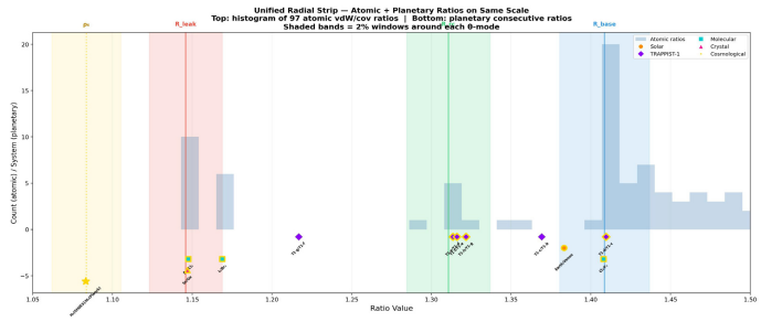
Figure 7: A Single Radial Axis Uniting All Scales. Top: Atomic Histogram. Bottom: Planetary, molecular, and Crystal Markers at Their Measured Ratios. The 2% Shaded Bands Capture the Majority of Cross-Scale Hits

Figure 8: Twin Top-Down Vortex Views: Atoms (left) and Planets (right) Mapped onto the Same Three Concentric, φ-Spaced Shells

How to Kill This Theory

Every claim in this paper can be destroyed by data. We welcome the attempt.

Prediction	Confirms if	Kills if	Data source
ρ6 = Hubble tension	Hº ratio stays 1.08 ± 0.01	Tension resolves below 2%	DESI + CMB-S4
M-dwarf peak at 1.41	TESS histogram peaks there	Peak at 1.31 or elsewhere	TESS DR3+
FGK peak at 1.31	Stays dominant	Shifts significantly	Kepler updates
TRAPPIST d/c = R_base	JWST refines to 1.409 ± 0.002	Shifts outside [1.40, 1.42]	JWST transit timing
Three modes universal	New systems show same 3 values	Different quantization appears	Any new dataset
Shell gap = 1/φ	Inner/total gap stays 0.62 ± 0.02	Ratio outside [0.60, 0.64]	Improved vdW data
Exponent m = 1/2	All elements keep Pythagorean form	Any element needs m ≠ 1/2	Atomic spectroscopy
Fib remainder = anomaly	Superheavy Fib-remainder has irregular config	Regular config at Fib remainder	Future element synthesis

The Strongest Near-Term Test is the TESS M-Dwarf Prediction.

Computational Tools and LLM Disclosure

All eigenvalue computations used Python 3 with NumPy, SciPy, and JAX (Metal GPU backend on Apple M4). Monte Carlo tests (100,000 random frameworks × 68 targets × 36,000 combinations) were GPU-parallelized. Formula discovery and adversarial testing were assisted by Claude (Anthropic) and Grok (xAI). All LLM-assisted steps were independently verified by direct numerical evaluation. LLMs are not listed as authors [1-16].

Data Availability

All code, eigenvalue tables, Monte Carlo results, and verification scripts are publicly available at: github.com/thusmann5327/ Unified_Theory_Physics.

References

1. Husmann, T. A. (2026). The Bigolloφ Method: A Pythagorean Unification of Atomic Radius Ratios via the Discriminant Triangle. Research Square.
2. Damanik, D., Gorodetski, A., & Yessen, W. (2016). The fibonacci hamiltonian. Inventiones mathematicae, 206(3), 629-692.
3. Maciá, E. (2017). Clustering resonance effects in the electronic energy spectrum of tridiagonal Fibonacci quasicrystals. physica status solidi (b), 254(10), 1700078.
4. Jagannathan, A. (2021). The Fibonacci quasicrystal: Case study of hidden dimensions and multifractality. Reviews of Modern Physics, 93(4), 045001.
5. Li, Z., & Boyle, L. (2023). The Penrose tiling is a quantum error-correcting code. arXiv preprint arXiv:2311.13040.
6. Bellissard, J. (1992). Gap labelling theorems for Schrödinger operators. In From number theory to physics (pp. 538-630).Berlin, Heidelberg: Springer Berlin Heidelberg.
7. He, M. Y., Ford, E. B., Ragozzine, D., & Carrera, D. (2020). Architectures of exoplanetary systems. III. Eccentricity and mutual inclination distributions of AMD-stable planetary systems. The Astronomical Journal, 160(6), 276.
8. Gilbert, G. J., & Fabrycky, D. C. (2020). An information theoretic framework for classifying exoplanetary system architectures. The Astronomical Journal, 159(6), 281.
9. Steffen, J. H., & Hwang, J. A. (2015). The period ratio distribution of Kepler's candidate multiplanet systems. Monthly Notices of the Royal Astronomical Society, 448(2), 1956-1972.
10. Agol, E., Dorn, C., Grimm, S. L., Turbet, M., Ducrot, E., Delrez, L., ... & Grootel, V. V. (2021). Refining the transit-timing and photometric analysis of TRAPPIST-1: masses, radii, densities, dynamics, and ephemerides. The planetary science journal, 2(1), 1.
11. Riess, A. G., Yuan, W., Macri, L. M., Scolnic, D., Brout, D., Casertano, S., ... & Zheng, W. (2022). A comprehensive measurement of the local value of the Hubble constant with 1 km s− 1 Mpc− 1 uncertainty from the Hubble Space Telescope and the SH0ES team. The Astrophysical journal letters, 934(1), L7.
12. Aghanim, N., Akrami, Y., Arroja, F., Ashdown, M., Aumont, J., Baccigalupi, C., ... & Pettorino, V. (2020). Planck 2018 results-I. Overview and the cosmological legacy of Planck. Astronomy & Astrophysics, 641, A1.
13. Huber, K. P. (1979). Constants of diatomicmolecules. Molecular spectra and molecular structure, 4, 146-291.
14. Kittel, C. (2005). Solid State Physics, 8th ed. Hoboken.
15. Alvarez, S. (2013). A cartography of the van der Waals territories. Dalton Transactions, 42(24), 8617-8636.
16. Sigler, L. (2002). Notes for Liber abaci. In Fibonacci’s Liber Abaci: A Translation into Modern English of Leonardo Pisano’s Book of Calculation (pp. 617-633). New York, NY: Springer New York