Techniques in Convolutional Depth Measurements

Problem Statement

In our laboratory, we are involved in a wide array of research and development activities that require specialized methods for measuring focus with high precision. Our work is interdisciplinary and ranges from the field of electro-optical (EO) engineering, robotics and radio-frequency (RF) imaging.

In the realm of electro-optical instruments, our efforts are primarily centered on the development and optimization of auto-focusing mechanisms. These systems are designed to adjust the focus automatically based on specific optical criteria, thus enhancing the quality and reliability of image or signal capture. Such auto-focusing capabilities are especially vital in applications where manual adjustment is impractical or where rapid, dynamic changes in focus are needed.

Simultaneously, we are also exploring the utilization of focus metrics within the context of radio-frequency domains. This involves developing algorithms and models that can interpret and analyze the RF signals to extract critical depth information. Here, the focus is not so much on visual images but rather on understanding the characteristics of emitting sources in RF environments. This information is invaluable in applications ranging from telecommunications to radar and navigation systems.

In the field of robotics, utilizing focal metrics to gauge depth presents an economical and convenient method for sensing the external environment. This form of depth sensing can be deployed for various applications, including navigational assistance and the creation of three-dimensional spatial models of areas traversed by the robot.

One method that we often employ across multiple projects is something akin to focal stacking. In this technique, multiple focal data points are collected and aggregated over a specific area of interest. This data collection allows us to construct a comprehensive depth map of the target, whether it be a physical surface in optical applications or an emitting source in RF contexts. The depth map generated offers a detailed, multi-dimensional representation of the area under study, and it provides invaluable data for downstream applications such as image reconstruction, target identification, and signal optimization.

The overarching objective of this research endeavor is to pinpoint a unified methodology for assessing focus that can be universally applied across ElectroOptical (EO) instrumentation as well as Radio-Frequency (RF) emission systems. The rationale for pursuing a solitary optimal technique is to streamline the allocation of developmental resources, thereby permitting concentrated investment in a single, multifaceted asset with wide applicability. By consolidating the focus measurement approaches for these disparate technologies into one unified system, we aim to achieve economies of scale and scope. This consolidation could facilitate a more effective allocation of human capital and financial resources, thereby expediting progress in each respective field.

Background

In the context of our Radio-Frequency (RF) research, one of the central components we employ is an image-forming antenna array. An antenna array is a composite system made up of individual antennas positioned in a specific geometric arrangement. When it comes to capturing depth information, this array operates somewhat analogously to a lens in an ElectroOptical (EO) system. Through advanced signal processing techniques, the antenna array produces images from the received RF signals, thereby converting the information from the electromagnetic spectrum to a spatial representation that can be more readily analyzed.

Interestingly, our focus measurements in RF systems have reached a level of sophistication where they are functionally equivalent to those in EO systems. This means that the methodologies for assessing focus— and thus depth information—can essentially be transposed from one system to the other. The criteria for evaluating the quality of focus in RF, such as resolution and signal-to-noise ratio, have corresponding parameters in EO, like sharpness and contrast. This functional equivalence lays the groundwork for our ambition to develop a universal focus measurement methodology.

The functional equivalence between EO and RF focus measurements offers several advantages. First, it simplifies the task of data interpretation, as analysts familiar with one system can more easily understand data from the other. Second, it permits a unified approach to algorithm development, thereby streamlining the research process. The ability to apply similar analytical frameworks to both EO and RF systems could lead to cross-disciplinary breakthroughs and may facilitate the optimization of focus measurement algorithms that are universally applicable.

The wavelengths employed in RF technologies differ markedly from those in EO systems. These disparities have a considerable impact on various aspects such as material interaction, signal propagation through space, and susceptibility to environmental factors. Nevertheless, the adverse effects arising from these intrinsic properties are mitigated through the strategic employment of narrow-band, piecewise frequency selection and the incorporation of directionality in the formation of images. Additionally, antenna polarization can be tailored to minimize signals that are reflected or otherwise unwanted.

Focal Stacking

The earliest applications of focal stacking were predominantly in the field of microscopy, where the objective was to capture a complete and focused view of three-dimensional biological samples. The derivation of depth information from these stacked images was a natural extension and became essential in scientific disciplines requiring detailed 3D reconstructions, such as cellular biology and materials science.

The process of measuring sharpness is central to focal stacking and subsequent depth extraction. The efficiency and accuracy of this process are highly reliant on the precise measurement of image sharpness at each focal plane. It is through the determination of maximal sharpness that applicable stack depths are identified.

Additional Applications

EO

In addition to depth calculations, there are a variety of other useful features of focal measure in EO that we make use of [1].

These metrics can also assist in object identification and segmentation. By understanding the areas of an image that are in focus, object recognition algorithms can better distinguish between the foreground and the background. While this is effectively an extension of depth measure, there is no specific production of depth maps, and it is not for the purpose of depth map generation. In dynamic settings such as video capture, changes in focal metrics over time can indicate the motion of objects. This becomes particularly useful in applications like security and optical declutter.

The quality of optical components, like lenses, can also be assessed through these metrics. They can determine how well an optical system can bring an image into focus. In projection with calibrated lenses, this allows for the measurement of projection surface quality.

In adaptive imaging systems that require real-time focus adjustments, focal metrics can provide the necessary data to dynamically adapt the focus. This is particularly relevant in situations where manual focus adjustment is either impractical or impossible, such as rapid projection setup, projection onto moving surfaces, or adjustment of cameras in similar situations.

In material analysis, focal metrics can provide valuable information on the texture and surface properties of materials. They offer different insights into material characteristics at various focal levels.

The metrics can serve as a robust tool for anomaly detection. Any unexpected variation in focus can signal either equipment malfunction or the presence of an obstructing object in the scene.

RF

As with EO, there are a variety of other useful features of focal measure in RF that we capitalize on. Focal metrics can identify Signal-to-Noise Ratio (SNR), which is a crucial metric that measures the level of a desired signal to the level of background noise. A higher SNR usually translates to better data integrity and less required error correction. It is also a valuable indicator of the performance of our bandpass filters and amplifiers.

Frequency stability can be tracked with focal metrics, which measure how well an emissions source maintains its frequency over time, including under varying environmental conditions. Frequency stability is useful as a device signature and can be especially useful in determining consumer versus military emissions.

Diffraction of signal power resulting from the insertion of an occluder in a signal path can yield valuable depth information.

Although beyond the scope of this article, finely detailed focus metrics in diffraction patterns can help identify the geometric characteristics of the diffracting occluder. This drifts into ptychography where focal metrics are used for quantitative phase imaging and beam characterization and holds considerable promise in RF [2].

The origins of phase noise in an oscillator circuit are influenced by many variables, including component tolerances, material properties, and even environmental conditions during manufacturing. As a result, devices of the same make and model can exhibit subtle differences in their phase noise profiles, and this noise can be measured using focal techniques as an extension of specialized SNR measurements on highresolution phase noise profiles.

Research Objectives

The primary goal here is to determine a depth map based on sharpness calculations of a focal stack, produced in a variety of ways.

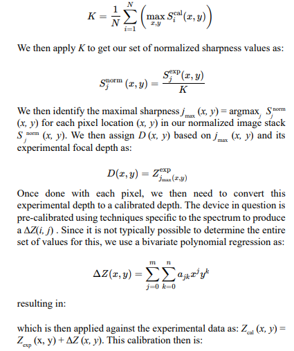
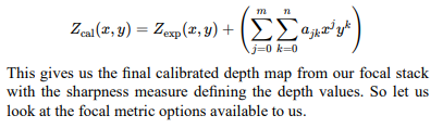
This depth map D (x, y) is comprised of the depth at each pixel based on a set of experimental input source images I_j^exp (x,y) where j is the specific image in the stack [2]. So, for each pixel (x, y) in an image, j we compute the sharpness value S_j^exp (x, y). For all pixels through all images, we normalize the sharpness values using a normalization constant K as:

Contrast Based Methods

Sobel Convolution

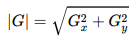
The Sobel gradient magnitude is a fundamental component of the Sobel operator, which, as previously mentioned, was developed by Irwin Sobel and Gary Feldman at the Stanford Artificial Intelligence Project in the late 1960s3. The Sobel gradient magnitude is essentially a measure of edge strength in an image and is computed from the horizontal and vertical gradients produced by the Sobel operator. It is not strictly speaking a focal function, but the gradient magnitude is an indicator of sharpness [3].

The Sobel gradient magnitude is an important construct because it gives a comprehensive measure of edge strength, taking into account variations in both horizontal and vertical directions. It provides a single scalar value that represents the "amount of edge" at each pixel, thereby simplifying the image for further analysis. This is particularly useful in edge detection, segmentation, and other image-processing tasks where the identification of boundaries is crucial.

Historically, the calculation of the Sobel gradient magnitude served as a computationally efficient way to approximate the true gradient magnitude in the days of limited computational power.Today, despite the availability of more sophisticated methods and far greater computational resources, the Sobel gradient magnitude continues to be widely used due to its efficiency, effectiveness, and ease of implementation.

The concept has been extensively utilized not only in traditional computer vision tasks but also in modern machine learning models as a feature extraction step or preprocessing stage. It serves as a fundamental building block in more advanced algorithms, including Canny edge detection, which itself uses gradient magnitude as a crucial step. The Sobel gradient magnitude has been an integral part of image processing and computer vision for over half a century.

Mathematically, the Sobel operation involves specialized convolving of the image f (x, y) with two separate 3x3 kernels, Gx and Gy , with one estimating the greatest horizontal gradient, and the other estimating the vertical gradient.

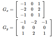
The resulting approximations, Gx and Gy are combined to determine the overall gradient magnitude of the image at each point using:

Laplacian Variance

The Laplacian Variance method for focus measurement is rooted in the mathematical theory of secondorder partial derivatives, commonly referred to as the Laplacian operator. The Laplacian operator is a wellknown tool in mathematics, physics, and engineering for assessing how a function changes relative to its mean. In the realm of image processing, it has become instrumental in edge detection, image enhancement, and other similar applications. Its origins in image processing appear to have been for sharpening, rather than focal metrology [4].

The concept of using Laplacian Variance as a focus measure is predicated on the idea that a well-focused image exhibits a high level of detail, translating to high-frequency components or sharp edges. Thus, by applying the Laplacian operator to an image and then calculating the variance (or standard deviation) of the resulting values, one gets a scalar metric that quantifies the image's focus or sharpness.

The Laplacian of an image is computed using a convolution operation with a specific Laplacian mask, often a 3x3 or 5x5 kernel, depending on the application requirements. The variance of the resulting Laplacian image then serves as the focus metric.

The Laplacian Variance method has gained prominence for several reasons. First, it's computationally efficient, much like the Tenengrad method. Second, it's versatile and robust against various types of noise. Because of these properties, Laplacian Variance has been adopted in various fields such as machine vision, robotics, and medical imaging. For instance, in automated microscopy where rapid and precise focusing is crucial, Laplacian Variance offers a dependable focus metric.

Its application extends to real-world commercial products as well, especially in the domain of consumer cameras and smartphones, where it is often used in autofocus algorithms due to its computational efficiency and effective performance.

In summary, the Laplacian Variance method for focus measurement has its foundation in classical mathematical operations and has evolved as an indispensable tool for several real-world applications requiring rapid and reliable focus assessment.

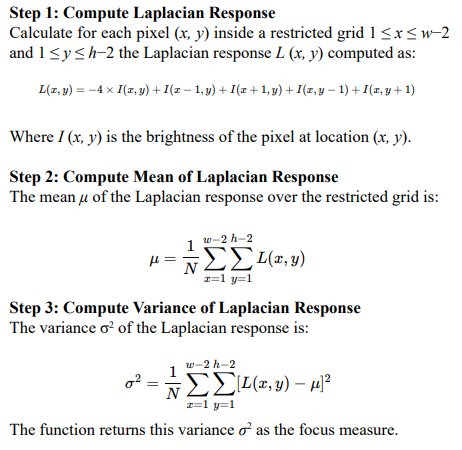
The Laplacian variance focus measure is calculated in three steps: first, by computing the Laplacian response for each pixel within the restricted area; second, by calculating the mean of these responses; and finally, by computing the variance of these Laplacian responses.

Where I is an image with dimensions w X h and the focus measure is computed over pixels to avoid border issues. So, then it also follows that N = (w−2) × (h−2).

Tenengrad Method

The Tenengrad focus measure was originally formulated as a sharpness metric based on the computation of image gradients. The term "Tenengrad" is a portmanteau of "Texture" and "Gradient," capturing the essence of the measure, which looks at the gradient magnitudes in an image to assess its sharpness or focus. While it's difficult to pinpoint exactly when or by whom the Tenengrad method was first coined, it has become a widely accepted measure for focus in the fields of computer vision, robotics, and microscopy, among others. The oldest reference I can find is Wang, 2007. The Tenengrad function gained attention for being computationally more efficient compared to some of the traditional methods, making it a go-to for real-time applications. The measure relies on the Sobel operator to calculate image gradients, a process that is computationally inexpensive and relatively easy to implement. Sobel operators have been used in image processing since they were introduced by Irwin Sobel and Gary Feldman in 1968, and are fundamental to edge detection techniques. The Sobel gradient magnitude provides a good approximation of the rate of intensity change in an image, making it a natural choice for assessing focus or sharpness.

Let's begin with definitions of Gx = Sobel operator for horizontal gradients, defined as [[ −1,0,1], [−2,0,2], [−1,0,1]] and Gy= Sobel operator for vertical gradients, defined as [[−1,−2,−1],[0,0,0],[1,2,1]]. The focus Measure = A cumulative value representing the focus measure of the image and pixels2D = A 2D array representing the grayscale values of each pixel in the image. Then for each pixel (x, y) in the imaging (while avoiding the borders), we calculate the gradients sumX and sumY by applying the Sobel operator:

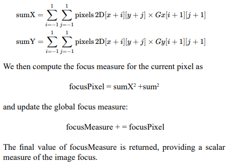
Image Analysis Methods

Histogram Method The use of histograms for gradient measurement has its roots in early work in computer vision and image processing, although the precise chronology might be less clearly delineated compared to more specific algorithms like the Sobel operator. One fascinating paper was on the automated underwater detection of crabs . The basic idea is to quantify edge strength or texture across an image or a region within an image by accumulating gradient magnitudes or orientations into a histogram [5]. This approach has found numerous applications, particularly in object recognition, texture analysis, and image segmentation.

Historically, the use of histograms in image processing predates many of the digital techniques commonly used today. In earlier times, histograms were used primarily for tasks like brightness and contrast adjustment. The extension to use histograms for gradient measurement gained prominence with the rise of more advanced image analysis tasks. For example, in object recognition, SIFT (Scale-Invariant Feature Transform) descriptors often employ histograms of oriented gradients (HOG) to describe local shape information. Developed by David Lowe in 1999, SIFT uses gradient histograms as a form of local feature descriptor that remains invariant to image scaling, orientation, and partially invariant to illumination changes.

Gradient histograms can provide a robust summary of an image or image region's local structure. In edge detection and texture discrimination tasks, a histogram of gradient magnitudes can serve to distinguish between different types of edges or textures. The approach has also been incorporated into machine learning algorithms to create feature vectors for image classification tasks. Histogram-based gradient measurement methods often offer a level of robustness against small transformations or deformations in the image, making them ideal for real-world applications where these types of changes are commonplace.

Furthermore, the efficiency of computing histograms makes these methods computationally attractive, facilitating their use in real¬time applications. In addition, the histogram-based approach easily lends itself to parallelization, making it highly efficient on modern hardware architectures.

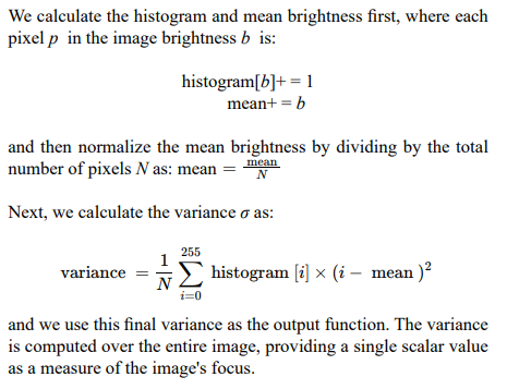
For this work, the histogram gradient calculates the variance of the brightness levels of an image, which can be used as a measure of focus or sharpness. We calculate the histogram and mean brightness first, where each pixel p in the image brightness b is:

Fourier Analysis

The Fourier Transform, formulated in the early 19th century by Joseph Fourier, has long been an essential tool in various scientific disciplines, including engineering, physics, and mathematics. However, its application to gradient analysis in image processing and computer vision can be considered a relatively modern development, gaining prominence in the latter half of the 20th century with the advent of digital computing. Some early use was in mask precision in integrated circuit manufacture and x-ray imaging.

The Fourier Transform provides a representation of a function, such as an image, in the frequency domain, allowing one to analyze different frequency components separately. This frequency-domain analysis is particularly powerful for understanding spatial relationships within an image, which naturally lends itself to gradient analysis [6-8].

In traditional image analysis tasks, like edge detection, the Fourier Transform is sometimes applied to analyze the frequency content of an image, since edges and fine details manifest as high-frequency components. By scrutinizing these high-frequency components, one can identify the existence, orientation, and even the quality of edges, which is a form of gradient analysis. Fourier-based techniques are often contrasted with spatial domain methods like Sobel or Canny edge detection, which perform similar tasks but in a different computational space.

Fourier analysis for gradient estimation gained academic attention in the late 20th century, with seminal papers providing foundational approaches for utilizing Fourier methods in image reconstruction and feature extraction. The approach has been found especially useful in scientific imaging techniques like MRI and CT scans, where the Fourier Transform plays a critical role in data acquisition and reconstruction algorithms. In these contexts, gradient analysis is crucial for feature identification and noise reduction.

The benefits of using Fourier Transform for gradient analysis include its suitability for analytical treatment and the ability to work in a transformed space where convolution operations, common in gradient analysis, are simplified to multiplication operations. However, Fourier methods usually require the entire image to be transformed, which may not be efficient for realtime or localized gradient analysis tasks.

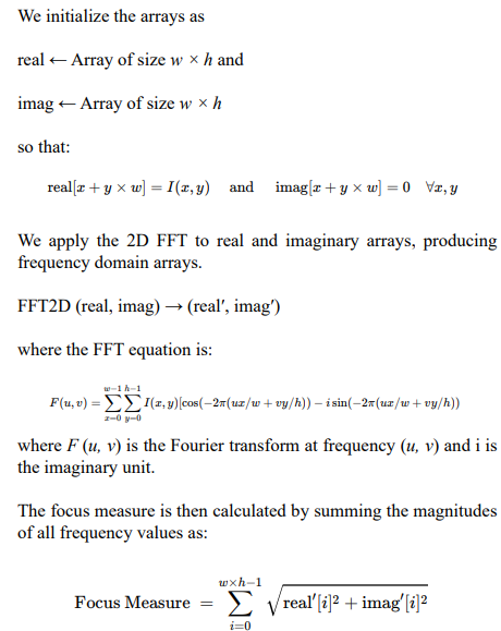
For these tasks, alternative methods such as wavelet transform might be more appropriate. For this implementation, we represent the given image I with dimensions w × h . The image is considered a 2D function where x , y are the spatial coordinates and I (x,y) the brightness at that coordinate.

Haar Wavelet Transform

The Haar Transform, named after its inventor, Alfréd Haar, was introduced in the early 20th century, around 1909. Originally conceived as an alternative to the Fourier Transform, the Haar Transform provides a method for representing functions in terms of a series of step functions. It was one of the earliest techniques in the development of wavelet theory and has been used for stock market price predictions (with limited success), image content analysis , and focal metrics, such as sex determination from retinal images [9, 10].

In the context of gradient analysis, the Haar Transform offers a computationally efficient way to capture abrupt changes in a signal, which aligns well with the identification of edges or rapid transitions in an image or dataset. Its utility in image and signal processing gained prominence during the 1980s and 1990s, particularly with the surge in wavelet research spearheaded by academics like Ingrid Daubechies and Yves Meyer. These developments were integral to the broader application of wavelet-based methods, including the Haar Transform, in gradient analysis, compression, and feature extraction.

The Haar Transform is especially effective at localizing features in both time and frequency, which makes it an attractive option for gradient analysis. This contrasts with the Fourier Transform, which is global in nature and less adept at capturing localized, transient features. Given its ability to provide sparse representations of signals and images, the Haar Transform has been employed in a variety of applications ranging from image compression algorithms like JPEG2000 to machine learning techniques for feature extraction.

Specifically, in gradient analysis, the Haar wavelets can detect sudden changes or discontinuities in a signal or image. This property can be useful in edge detection, texture discrimination, and other tasks where the gradient or rate of change is of interest. The coefficients produced by the Haar Transform can effectively summarize how much a function changes at different scales and at different points, making it a powerful tool for gradient analysis.

Because of its simplicity and lower computational complexity compared to other wavelet transforms, the Haar Transform is often chosen for real-time applications and embedded systems where computational resources are limited. However, its simplicity also comes with limitations, such as less smooth wavelet functions compared to other wavelets like Daubechies wavelets.

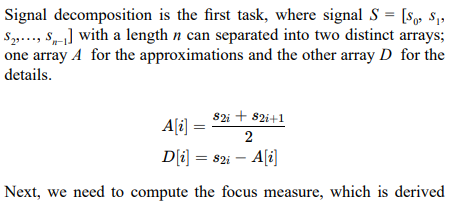
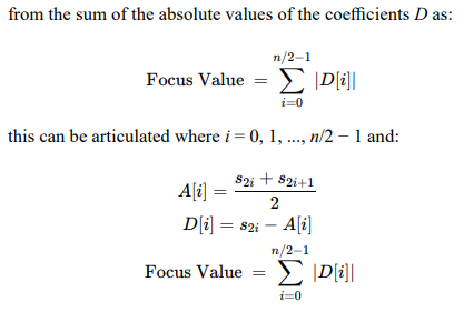
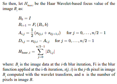
The Haar wavelet transform dissects a signal into a pair of coefficient sets: one for approximation and the other for details.

Normalization

In order to plot all the values next to one another to see linearity and general behavior, all the focus measures for each of the 100 examples are normalized [11]. We start by finding the minimum and maximum values of the array, calculate the range and then normalize as:

Scope and Limitations

The primary objective of this research is to generalize the results to various segments of the electromagnetic spectrum, inclusive of radio frequencies (RF). In this paper, experimental evaluations are confined to the optical spectrum, serving as an initial approximation for anticipated outcomes in other spectral regions, based on the RF image formation rationale described already. The present work abstains from examining the nuances related to wavelength variability and the influence of wave interactions at lower frequencies; these issues are designated for exploration in subsequent investigations.

Research Design

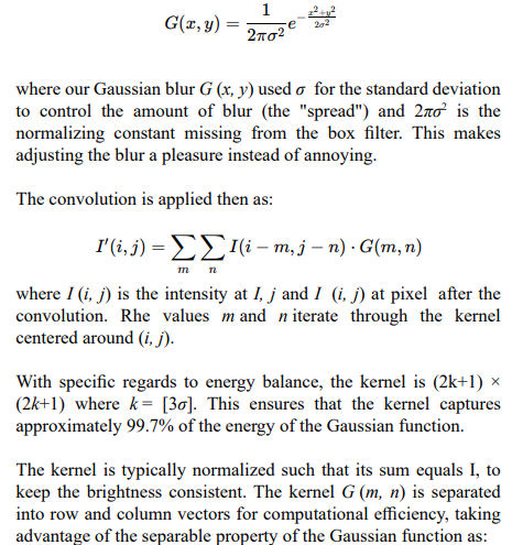
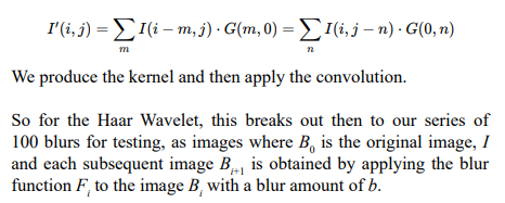
Data Examples A limitation of the proposed solution is the use of stepper motors in certain projects. When operating these stepper motors to achieve precise focusing, the direction towards optimal focus should ideally be unambiguous at all points along the focal metric curve. Consequently, the desired behavior is a linear response that does not exhibit any changes in the direction of the curve. Also, the curve slope will ideally not go flat anywhere, creating ambiguity. Furthermore, it is desirable that the curve slope remains non-zero throughout to avoid any regions of ambiguity or narrow precision. For the evaluation phase, I've selected a variety of images to assess the performance of these algorithms under diverse scenarios. The initial test employs a straightforward checkerboard design, which serves as an optimal subject for focus assessment. The subsequent image features a wax sculpture, offering a more realistic depiction of the kinds of subjects the system is expected to encounter, particularly in the optical spectrum. The final image is one with low contrast, posing a complex challenge for focus-determination algorithms. The evaluations were configured in two distinct modes—coarse focus and fine focus—to assess the algorithms' adeptness at managing both minor and major focus adjustments. The objective is to confirm that the algorithms exhibit both sensitivity and specificity; they should be proficient in identifying subtle focus shifts while minimizing ambiguity across both scales. By testing with a range of examples, I aim to find an algorithm that is both effective and reliable across a range of different imaging conditions. This is important for ensuring the system's practical usefulness, in addition to its overall validity. Blur For these tests, I applied a blur to the original images. Interestingly, for fine blur adjustments, box convolutions felt unwieldy while trying to maintain balanced energy. As such, I moved to a Gaussian blur as:

Data Analysis

Results

The two datasets, coarse and fine, both provide useful clues as to the appropriateness of each function. The histogram method was unstable and produced metric curves that exhibited changes in slope direction. This is problematic for servos and motors. The Laplacian Variance exhibited insufficient gradient when the subject was not in near-perfect focus. This poses a challenge for focus optimization, as the metric becomes less informative about the degree to which the subject is out of focus.

The Haar and Fourier techniques produced outcomes that were strikingly similar, despite their different approaches to frequency component analysis. Specifically, while the Fourier method offers a comprehensive frequency representation of the image, the Haar approach provides a more rudimentary, coarse-grained decomposition. Unexpected was that the Fourier method was slightly faster than Haar, despite being generally considered less precise. Either appears sufficient for reliable focus measurement. These minor variations in speed could easily represent artifacts in implementation, rather than inherent computational load.

The Tenengrad algorithm exhibited notable stability; however, it did present limitations concerning its slope in the fine-focus test, particularly when applied to low-contrast images. This is somewhat unexpected given the algorithm's prevalent use in autofocus systems for cameras. Lastly, the Sobel method's performance was notably robust, an outcome that is somewhat surprising given the algorithm's computational simplicity. The method seems to offer a satisfactory balance between computational efficiency and the capacity to provide meaningful focus metrics.

Conclusion

The methods that are the most computationally efficient unfortunately yield the least acceptable results, as evidenced by the accompanying illustration. While this outcome might not be entirely unexpected, it is worth noting. The focus metrics that performed the best share a similar level of computational burden, at least before any software optimization efforts. In the context of our work, these findings point towards the utility of the Haar method, although the Fourier and Sobel methods also present strong cases for consideration. On the other hand, the Histogram, Laplacian, and Tenengrad methods seem to be better suited for scenarios where the imagery under study is never significantly out of focus.

These results do not correlate with an earlier study , most likely due to different goals.

Future Work

A number of image classes were not tested. Significant open questions remain in high-noise imagery; which may involve speckle, compression, low resolution, and dynamic range artifacts [12].

Some of the significant open questions in high-noise imagery include:

1. Speckle: Speckle may refer to the granular noise caused by coherent imaging systems such as synthetic aperture imaging or night vision systems. It also refers to high-frequency noise in EO imagery. Open questions in this area include methods to accurately remove the speckle, to prevent focus metrics from using them, while preserving important image details.

2. Compression artifacts: Blocking, ringing, moire, quantization errors and posterization are some common examples. Each of thee has the potential to bias, or at least mute, the focal metric.

3. Low resolution: Low-resolution images lack fine details and can adversely affect various applications, such as target recognition or object detection. Open questions in this area involve improving resolution enhancement techniques, exploring super-resolution algorithms, or leveraging deep learning approaches to recover finer details from low-resolution images. The big open issue is if methods such as super-resolution algorithms damage depth prediction, despite how pleasant the image may appear.

4. Dynamic range artifacts: High-noise imagery can suffer from limited dynamic range, resulting in loss of details in bright or dark regions. Open questions include developing better techniques for dynamic range recovery for compression and expansion, as well as exploring algorithms specifically tailored to handle high-noise data with a wide range of intensity values.

Addressing these open questions will help determine the possible depth effects of increasingly common AI-enhanced imagery.Also open are questions regarding the effect of geometric positioning within the image, especially with non-frequency domain methods. The impact of edge effects, object localization, aspect ratio, and anisotropic content needs exploration.

Lastly, the impact of imagery with rolling gradients, which are sometimes found in RF needs testing. Smooth gradients lack edges to measure and may require alternative techniques or enhancement such as contrast enhancement, more aggressive noise reduction, and investigation as to metric sensitivity to gradient changes.

Numerous other focal metrics exist, some of which incorporate machine learning algorithms. While there is a keen interest in evaluating these additional methods, the constraints of the current study are dictated by the available time for research, coding, and testing.

These will be the topics of future research.

         

Coarse Focus                                                                                       Compute Times

Fine Focus

References

1. Govil, A., Pallister, D., & Morris, M. (1993). Three-Dimensional Digital Confocal Raman Microscopy. Applied Spectroscopy, 47(1), 75-79.
2. Xin-Yu, P., Xiao-Xue, B., Zheng, D., Zhi, G., Han, X., Yi, Z., ... & Cheng-Long, Z. (2023). Review of development for ptychography algorithm. Acta physica sinica, 72(5).
3. Feldman, J. A., Feldman, G. M., Falk, G., Grape, G., Pearlman, J., Sobel, I., & Tenenbaum, J. M. (1969, May). The Stanford Hand-Eye Project. In IJCAI (pp. 521-526).
4. Strickland, R. N., & Aly, M. Y. (1985). Image sharpness enhancement using adaptive 3x3 convolution masks. Optical Engineering, 24(4), 683-686.
5. Wang, F. Y., WANG, R., & Zhang, G. J. (2007). Auto-focusing system based on DSP [J]. Opto-Electronic Engineering, 34(8), 134-138.
6. Cao, S., Zhao, D., Sun, Y., & Ruan, C. (2021). Learning-based low-illumination image enhancer for underwater live crab detection. ICES Journal of Marine Science, 78(3), 979-993.
7. Rosner, S. J., Shamma, N., & Sporon-Fiedler, F. (1994, May).Fourier analysis determination of best focus in submicron lithography. In Integrated Circuit Metrology, Inspection, and Process Control VIII (Vol. 2196, pp. 314-320). SPIE.
8. Shimakawa, Y., Nishiki, M., Yanagita, S., Nishikawa, N., Sakai, T., Ito, H., ... & Yanagawa, N. (2023). Evaluation of x-ray effective focal spot size dependency on x-ray exposure settings using edge response analysis. Radiological Physics and Technology, 16(1), 39-47.
9. Qiu, J., Wang, B., & Zhou, C. (2020). Forecasting stock prices with long-short term memory neural network based on attention mechanism. PloS one, 15(1), e0227222.
10. Kohrs, A., & Merialdo, B. (2001). Creating user-adapted Websites by the use of collaborative filtering. Interacting with Computers, 13(6), 695-716.
11. Berk, A., Ozturan, G., Delavari, P., Maberley, D., Yilmaz, Ö., & Oruc, I. (2023). Learning from small data: Classifying sex from retinal images via deep learning. Plos one, 18(8), e0289211.
12. Shih, L. (2007, February). Autofocus survey: a comparison of algorithms. In Digital photography III (Vol. 6502, pp. 90-100). SPIE.