Introduction

The characterization of sediments plays a vital role in understanding environmental processes, assessing pollution levels, and managing natural resources. Techniques such as Energy Dispersive X-ray Fluorescence (EDXRF), X-ray Diffraction (XRD), and Fourier Transform Infrared Spectroscopy (FTIR) have gained prominence in sediment analysis due to their sensitivity, accuracy, and ability to provide detailed compositional information. This current literature on these methods highlights their applications, advantages, and limitations in sediment characterization. emphasized EDXRF as being widely used for the elemental analysis of sediments due to its ability to identify heavy metals and trace elements with minimal sample preparation. Recent studies have demonstrated the effectiveness of EDXRF in detecting pollutants, especially in contaminated marine and riverine sediments. For instance, research conducted highlighted the utility of EDXRF in assessing metal concentrations in river sediments impacted by industrial discharges [1]. The study reported that the method provided reliable quantitative data, allowing for the identification of pollution hotspots.

Moreover, EDXRF's non-destructive nature allows for in-situ measurements, making it advantageous for field studies. However, the technique has limitations regarding its detection limits and matrix effects, which can hinder the analysis of lighter elements and compounds. The work emphasized the need for careful calibration and matrix matching to optimize results. X-ray Diffraction (XRD) is an essential tool for determining the mineralogical composition of sediments [1]. It provides insights into the crystalline structure, phase identification, and quantification of minerals. Recent advances in XRD technology, such as Multi-Detector XRD (MD- XRD), have improved the speed and accuracy of mineral analysis. For example, a study utilized MD-XRD to characterize mineral assemblages in river sediments, revealing significant variations in mineralogy influenced by sediment source and transport processes [1]. The combination of XRD with Rietveld refinement techniques has enabled researchers to achieve high accuracy in quantifying mineral phases. However, XRD is limited by its inability to detect non-crystalline materials, meaning approaches such as FTIR or complementary analyses are often required for a comprehensive characterization. Further studies have shown that Fourier Transform Infrared Spectroscopy (FTIR) is adept at identifying organic compounds and functional groups in sediments, making it particularly useful for studying organic pollutants and biomaterials. Recent studies, like that of have shown that FTIR can effectively characterize organic matter in sediments and assess changes due to environmental factors or anthropogenic influences [2].

This technique has also been combined with EDXRF and XRD to provide a holistic view of sediment composition. FTIR's sensitivity to moisture content can be a double-edged sword; while it allows for the analysis of water-rich samples, it can also introduce variability in results. Studies have advocated for the standardization of sample preparation methods to mitigate this issue [3]. In the Integrated Approaches, the integration of EDXRF, XRD, and FTIR offers a powerful approach for comprehensive sediment characterization. Current literature increasingly supports multidimensional analysis, as evidenced by research combining these techniques to paint a detailed picture of sediment composition.

For instance, a joint study highlighted the effectiveness of using EDXRF for elemental analysis, XRD for mineralogical identification, and FTIR for organic characterization, demonstrating significant correlations that reflected both natural processes and anthropogenic impacts on sediment quality [4]. Conclusion: The combination of EDXRF, XRD, and FTIR has significantly enhanced the understanding of sediment composition and quality. Each technique offers unique strengths, and their integration allows for a more comprehensive analysis and understanding of sediment characteristics. However, researchers must remain aware of the limitations inherent to each method and strive for standardized practices to ensure the accuracy and reliability of results. Future research should focus on developing standardized protocols for data integration and interpretation, enhancing both the efficiency and precision of sediment characterization studies.

Materials & Methods

Study Area

                                                         Table 1: Shown the Sampling Locations of the Dumpsites

Location and Historical Background of the Study Area

This study was conducted in Ilorin Metropolis, the capital of Kwara State. The city is situated in the traditional zone between Nigeria's forest and savannah regions and serves as the gateway city between northern and southwestern Nigeria (Ogunsanya, 1984; Oyebanji, 1993) and the sampling locations, Latitude (N) and Longitude (E) and tabulated in table 1.

Figure 1: Map of Kwara State Shown the University of Ilorin Dumpsites (Source: Satellite Imaging)

Collection and Pre-Treatment of Samples from Sampling Points

Three 'government-approved' dumpsites comprising two active and one abandoned in Ilorin. The three dumpsites are shown in Figures 1 as map of Kwara state with the three dumpsites imbedded in the map and another figures 2, 3 and 4 representing Pictorial View of the University of Ilorin dumpsite (Active), Gbagede dumpsite (Active), and Ogundele dumpsite (Abandoned). As a first preparation step before XRD, EDXRF, and FTIR analysis, sediment samples were oven-dried at 105â??, cooled, homogenized by grinding, and sieved through a 2 mm mesh size sieve before being further sub-sampled and labeled in plastic vials. Before FTIR analysis, 2 mg of the crushed sand was mixed carefully with 198 mg of dry potassium bromide (KBr). The mixture was then compressed to form a pellet of 13 mm diameter and 1 mm thickness. Agilent Technology Cary 630 FTIR running under higher frequency was allowed to pass through Standard Operating Procedures starting from sampling operation to cleaning operation using organic solvent before 10 - 15 mg of solid sediment samples were placed on the KBr cell and pressed to make a pellet on top of the crystal before the constituents' bonds of the sediment samples were obtained.

For X-ray fluorescence measurements, the crushed sample was compressed under high pressure for a few minutes to form a measurable pellet. An Oxford EDXRF instrument with model No. X-Supreme 8000 EDXRF was used to measure the processed and crushed sediment samples, which were compressed under high pressure for seven minutes to form a measurable pellet. Then, the system was shut down to convert the intensities into mg/kg or weight percentage concentrations and carry out the measurements. To determine the crystallographic structures of the sediment samples, we used X-ray powder diffraction. The crystallographic parameters of the sediment samples were determined using an XRD Benchtop powder refractometer with model Rigaku Miniflex 600 by Rigaku Corporation Japan at Ahmadu Bello University Zaria, Nigeria, at room temperature; the diffractometer works with a Two-Theta starting position at 4 degrees and ends at 75 degrees with a two-theta step of 0.026261 at 8.69 seconds per step with a current of 40 mA and a tension of 45 VA, to obtain different crystallographic structures such as Body-Centered Cubic Structure, Face-Centered Cubic Structure, and hexagonal close- packed structures.

Figure 2: University of Ilorin Dumpsite (Active) (Source: University of Ilorin Health & Environmental Services)

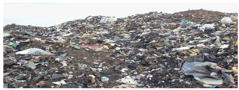
Figure 3: Gbagede Dumpsite (Active) (Source: Kwara State Ministry of Environment)

Figure 4: Ogundele Dumpsite (Abandoned) (Source: Kwara State Ministry of Environment)

Percentage Recovery

Undisturbed white soil samples were collected from Ilaro, Ogun State, Nigeria. The samples were made to undergo further processing after oven drying at 105â??. Before that, they were thoroughly acid-washed and rinsed several times with clean distilled water. The samples were allowed to cool after oven drying; the cooled samples were divided into two for digestion. One is tagged "spiked," while the other is an "unspiked" sample. The spiked samples are expected to contain 1 g of salt of Pb, Zn, Cu, Cd, Cr, and Fe at about 10 - 20 ppm standard solution, and the standard solution is expected to be 0, 10, 20, 30, 40, 50, … 100 ppm. Both the spiked and unspiked samples are digested using concentrated H₂SO₄ and H₂O₂ in the ratio 2:4. The experiment was repeated using concentrated HNO3 and HClO₄ to allow for comparison, and the digestion was performed using the standard approved method. The results of the spiked and unspiked samples are tabulated in tables 2 and 3 below, and the percentage recovery is determined.

                                                                                           Recovery = X 100

Table 2: Percentage Recovery for the Unspiked Samples

                                                        Table 3: The Percentage Recovery for the Spiked Samples

Spectroscopic Characterization of Sediment of the Studied Area by FTIR, XRF, and XRD Analysis

The chemical and crystal structural properties of sediments were carried out using a well-established analytical protocol [5]. Sample collection and preparation of sediment samples were conducted using a stainless sediment grab sampler at all designated locations during the dry and rainy seasons in 2018 and 2019 and labeled before being transported to the laboratory for further processing and analysis. The natural sediment was oven-dried in the laboratory at 120 â?? to remove the moisture content. Then the sediment was allowed to cool before being ground using a glass pestle and mortar and later sieved to obtain acceptable sediment samples of about 2 mm.

Standard Operating Procedures (SOP) for FTIR

a) The Agilent Technology Cary 630 was turned on and allowed to warm up for 10 - 15 minutes.

b) The computer attached to the FTIR was double-clicked after initialization on the Microlab PC window icon and waited to open.

c) The system was clicked again to initiate automatic sampling operation, and the method was selected in the form of absorbance or transmittance.

d) The crystal was cleaned with an organic solvent, and background information was obtained after the second click.

e) A solid sample of about 10 - 15 mg was placed on the cell and pressed to make a pellet on top of the crystal, but for liquid samples, it remained open to smear on top of the crystal and clicked next for the system to equilibrate.

f) Then the sample alignment check for the blue line changed from red to the green region and proper coding of the sample identity.

g) For the second sampling, the system was then clicked again, and right-clicked for picking the peaks and selecting peaks for proper labeling by dragging to acquire the wave numbers as well as transmittance or absorbance.

Analysis of Sediments Using FTIR

Agilent Technology Cary 630 FTIR running under higher frequency was allowed to pass through standard operating procedures starting from sampling operation to cleaning operation using an organic solvent before 10 - 15 mg of solid sediment samples were placed on the KBr cell and pressed to make a pellet on top of the crystal before the constituents' bonds of the sediment samples were obtained.

Standard Operating Procedures (SOP) for XRD

X-ray powder diffraction is most widely used to identify unknown crystalline materials (e.g., minerals and inorganic compounds). Determining unknown solids is critical to geology, environmental science, engineering, and biology studies with specialized techniques. XRD SOP: The XRD NGRL works with other components, like the water chiller, which cools the X-ray tube and maintains a uniform temperature. Then the air was compressed, which helps in opening and closing the cabinet door. The XRD machine was connected to the computer workstation using data collector software from Panalytical. The goniometer forms the central part of the Empyrean diffraction system with omega and 2theta axes. The sample stage diffracted beam optics, including the detector mounted in a specific position on the goniometer, which was in vertical mode, can be configured to analyze materials finely and bulk composition. Before then, the sample preparation occurred in a block and was compressed in the flat sample holder to create a flat, smooth surface later mounted on the sample stage in the XRD cabinet. The sample was analyzed using the reflection- transmission spinner stage using the theta-theta setting. The two- theta starting position was 4 degrees and ended at 75 degrees, with two-theta steps of 0.026261 at 8.67 seconds per step. The tube current was 40 mA, and the tension was 45 VA. A programmable divergent slit was used with a 5 mm width mask, and the gonio scan was used to obtain the intensity of diffracted X-rays continuously, and the computer system automatically records the results.

Analysis of Sediments Using XRD

The crystallographic parameters of the sediment samples were determined using an XRD benchtop powder refractometer with model Rigaku Minflex 600 by Rigaku Corporation Japan at Ahmadu Bello University Zaria Nigeria at room temperature; the diffractometer works with a two-theta starting position at 4 degrees and ends at 75 degrees with a two-theta step of 0.026261 at 8.69 seconds per step with a current of 40 mA and a tension of 45 VA.

Standard Operating Procedures (SOP) for EDXRF

The processed sediment samples were cleaned after cleaning the sample up, and the filter was fixed. The sample was then put in the clean sample cup so that the filter was covered at the bottom with a thickness of about 3 mm. Then the system was turned on and allowed to warm up for 30 minutes, selecting the appropriate method concerning the nature of the selected Sample and also to accept analytical reading, which occurs between 6 - 7 minutes. Then the x-ray is then shut down, the intensities are converted to concentration in mg/ kg or weight percentage, and the results are published or printed.

Analysis of Sediment Using EDXRF

An Oxford EDXRF instrument with model No X - Supreme 8000 XRF was used to measure when the processed and crushed sediment samples were compressed under high pressure for seven minutes to form a measurable pellet. Then, the system was shut down to convert the intensities into mg/kg or weight percentage concentrations.

Quality Control and Assurance for FTIR, EDXRD, and XRF:

Triplicate analysis of the samples was carried out to ensure the accuracy of the data generated from all the analytical equipment. The blank samples were analyzed at every ten determinations. Also, a working standard was run as a sample

Figure 5: Face – Centered Cubic Structure of Close Packed Adopted from Research Gate

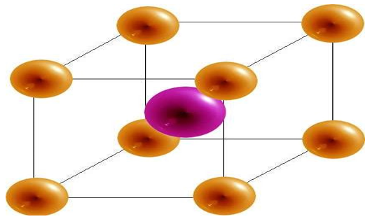
Figure 6: Cubic Lattices and Close Packing – Chemistry Called Body Center Structure Adopted from Research Gate

Figure 7: Hexagonal Closest Packed Adopted from Research Gate

The Figures 5, 6 and 7 exhibited the Face – Centered Cubic Structure, Body center cubic structure or Cubic Lattices and Close Packing and Hexagonal closed packed structures obtained from crystallography analysis of the sediments

Results & Discussion

Geochemical Properties of Sediment Using XRD, EDXRF, and FTIR

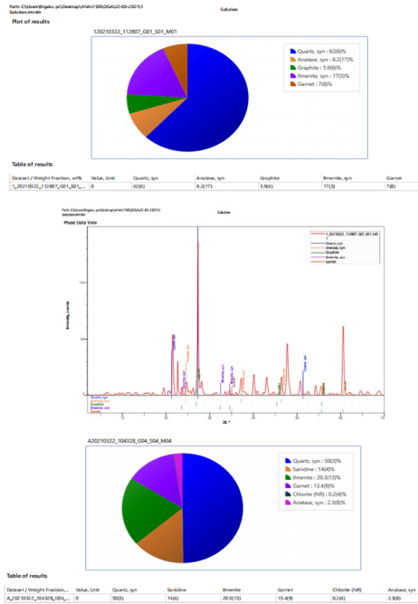
                                                     Table 4: Summary of Results of XRD Characterization of Sediment

The XRD Spectra and Pre-Chart for all the Sediment Samples are Shown in Appendix 2

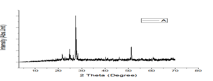
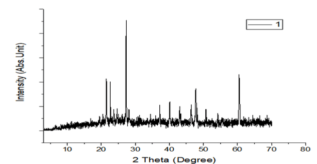
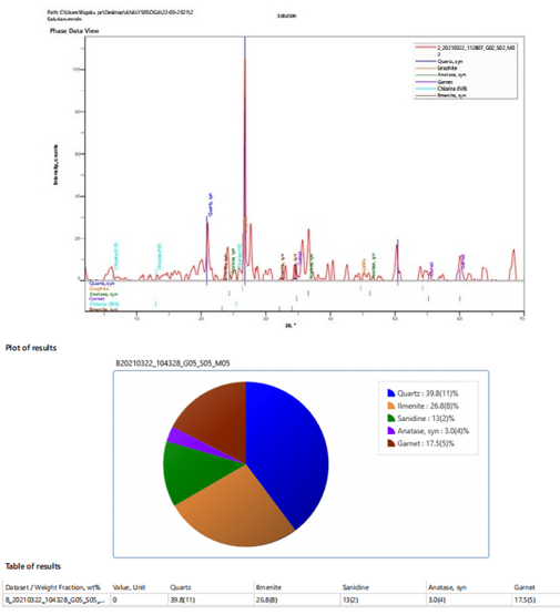
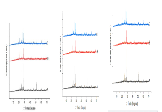
Figures 8: A, B, C: XRD Charts for 2018 and 2019 Dry Seasons and the Blank

Analysis of Sediments by X-Ray Diffraction (XRD)

The observed mineral phases in the sediment are summarized in Table 4 a better and further illustrated with figures 8 as the XRD Spectra and pre-chart for all the sediment samples as shown in Appendix 2 which are Quartz and anatase as abundant in the sediment enumerate in. table 4 and they are the most common minerals in the geosphere and are usually found in most geological environments. Ilmenite, chlorite, garnet, graphite, orthoclase, goethite, and sanidine are also found in these studies, and these minerals are of igneous, beach sand, clay, coal, and feldspar origin. The results are an indication of the enrichment of heavy metals embedded in the sediment as a result of runoff from the solid waste at the dumpsites and discharged into associated rivers and streams under this study, which brings about an increase in pollution indices such as enrichment factor, contamination factor, geoaccumulation, ecological risk, and potential ecological risk (PEER) or risk index. According to Mart Van Bracht, President of Euro Surveys in the geological study of Europe, minerals are naturally occurring substances with distinctive chemical and physical properties. They are the building blocks of the rock that forms the Earth. There are more than 4,500 recognized minerals; some are very common while others are uncommon, and most of them are used in society in a wide range of applications like construction, manufacturing, agriculture, and energy supply.

Table 5: Result of EDXRF for Sediments Obtained from Associated Lake and Stream at UI, OG, and GB Dumpsites in 2018 and 2019 dry and the Raining Seasons, Respectively

Table 6: Result of EDXRF for sediments obtained from associated 1000m upstream of UI, OG, and GB Dumpsites used as a control in 2018 and 2019 dry and Raining Seasons, respectively

The EDXRF Spectra and Pre-Chart for All the Sediment Samples Are Shown in Appendix 3

Figures 9: A, B, C: EDXRF Charts for 2018 and 2019 Dry Seasons and the Blank

Analysis of Sediment Using EDXRF

The EDXRF results are summarized in Tables 5 while table 6 served as control and a better illustration is further demonstrated inn figures 9 with the EDXRF Spectra and pre-chart for all the sediment samples as shown in Appendix 3 with the highest concentration of silica (65.768) and the lowest concentration of nickel oxide, cobalt oxide, and lanthanum III oxide (0.00). Also, deficient levels of other oxides were found in the sediment, as shown in Appendix 3 and Tables 4.82 to 4.84, with an insignificant amount of trace elements such as Fe, Cu, Zn, Ca, Ge, Lu, Ta, W, Hg, Mg, Al, Cl, K, Ti, V, Cr, Mn, and Ba. These results confirm that the sediments under this study consist mainly of quartz with little anatase and minor calcite, chlorite, garnet, and graphite. The low concentration of these oxides suggests partial purity of the sediment and shows that the EDXRF results agree with the XRD results.

Table 7: Observed IR Absorption Frequencies of Sediment Samples and their Assignments

The FTIR Spectra and Pre-Chart for all the Sediment Samples are Shown in Appendix 4

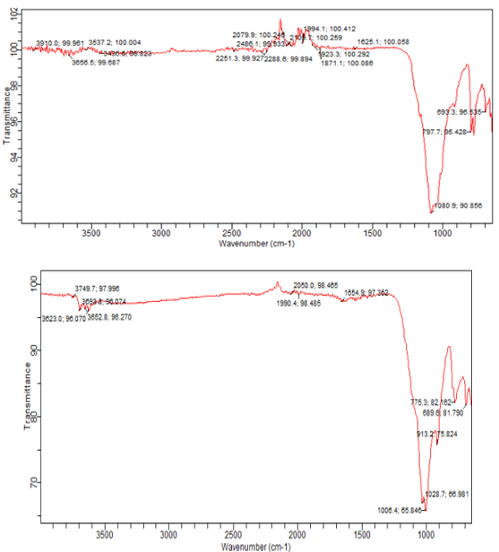
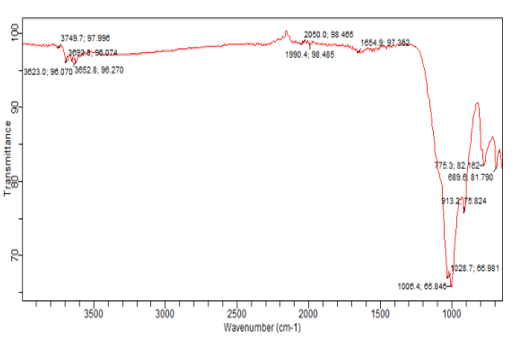
Figures 10: A, B, C: FTIR Charts for 2018/ 2019, the Blank and the Superimposed Charts Appendix 5

Analysis of Sediments by Fourier - Transform Infrared Spectroscopy (FTIR)

Figure 10 a, b, and c shows the qualitative analyses of the sediment samples using FTIR spectra which are carried out to determine the sediment samples' significant and minor organic and inorganic mineral constituents. The minerals are identified using the available literature. The positions of the observed absorption bands in wavenumber units are summarized in Table 7 with the FTIR typical and superimposed spectrum available in Appendix of the FTIR Spectra and pre-chart for all the sediment samples are shown in Appendix 4 and 5 with High-intensity absorption bands are observed at 3911 and 3656 as the main components of the sediment samples under this study; the regarded bands are due to stretching vibrations of water, hydroxyl, and organic alcohols. Less intense bands have also been observed at a wavenumber of 98.725 - 98.861, which are due to (CO₃)²^- asymmetric and symmetric stretching and Si-O-Si (symmetrical bending). The silica (Si-O- Si) vibration in the samples again confirms the presence of quartz. Other significant bands observed are 689.6 - 775.3, 909.5, and 1028.7, due to amino stretching or M-N stretching [6-14].

Acknowledgement

We express our genuine gratitude to all individuals who have directly and indirectly contributed to the success of these studies, especially my first son, who taught me the making of graphic abstracts. Your support and involvement have been instrumental in shaping the positive outcomes achieved in this research endeavor.

References

1. Shabbusharma. (2020). X-ray Diffraction Analysis PrincipleInstrument and Applications.
2. Ishii. (2019). Strategy for the Formation of Parametric Images Under Conditions of Low Injected Radioactivity Applied to PET Studies With the Irreversible Monoamine Oxidase A Tracers [11C] Clorgyline and Deuterium-Substituted [11C] Clorgyline; Journal of cerebral blood flow and metabolism: oficial journal of the International Society of Cerebral Blood Flow and Metabolism 22(11):1367-76
3. Ishii, K., Lyons, M. M., & Carr, S. A. (2019). Revisiting media richness theory for today and future. Human behavior and emerging technologies, 1(2), 124-131.
4. Liang, F., Yang, S., & Sun, C. (2011). Primary health risk analysis of metals in surface water of Taihu Lake, China. Bulletin of environmental contamination and toxicology, 87, 404-408.
5. Nassima. (2019). Assessment of heavy metal contamination status in sediments and Identification of pollution source in Ichkeul Lake and rivers ecosystem, northern Tunisia. Arabian Journal of Geosciences 9(9).
6. Chandramohan, J., Chandrasekaran, A., Jebakumar, J. P. P., Elango, G., & Ravisankar, R. (2018). Assessment of contamination by metals in coastal sediments from South East Coast of Tamil Nadu, India with statistical approach. Iranian Journal of Science and Technology, Transactions A: Science, 42, 1989-2004.
7. Hakanson, L. (1980). An ecological risk index for aquatic pollution control. A sedimentological approach. Water research, 14(8), 975-1001.
8. Krishna, A. K., Satyanarayanan, M., & Govil, P. K. (2009). Assessment of heavy metal pollution in water using multivariate statistical techniques in an industrial area: a case study from Patancheru, Medak District, Andhra Pradesh,India. Journal of hazardous materials, 167(1-3), 366-373.
9. Nouri, M. (2016). Assessment of metals contamination and ecological risk in ait Ammar abandoned iron mine soil, Morocco. Ekológia (bratislava), 35(1), 32-49.
10. Masri, S., LeBrón, A. M., Logue, M. D., Valencia, E., Ruiz, A., Reyes, A., & Wu, J. (2021). Risk assessment of soil heavy metal contamination at the census tract level in the city of Santa Ana, CA: implications for health and environmental justice. Environmental Science: Processes & Impacts, 23(6), 812-830.
11. Jeanger, R. R., Jeanger, P., Juanga., & Visvanahan, C. (2021). Dumpsite Toxicity Assessment and Potential for Rehabilitation (2022): A Case Study at Maung Pathum Dumpsite, Thailand, Journal of Environmental Engineering and ManagementProgram (1) 30-39
12. Sakan, S. M., devic, D. S., Manojlovic, D. D., & Predrag, P.S. (2009). Assessment of heavy metal pollutants accumulation in the Tisza river sediments. Journal of environmental management, 90(11), 3382-3390.
13. Sakan, S. M.,devic, D. S., & Trifunovic, S. S. (2011). Geochemical and statistical methods in the evaluation of trace elements contamination: an application on canal sediments. Pol. J. Environ. Stud, 20(1), 187-199.
14. Sekabira, K., Origa, H. O., Basamba, T. A., Mutumba, G., & Kakudidi, E. (2010). Assessment of heavy metal pollution in the urban stream sediments and its tributaries. International journal of environmental science & technology, 7, 435-446.