Spatial Air Quality Assessment in Peninsular Malaysia: Insights from Environmetric Analyses and Artificial Neural Networks

Introduction

Air quality degradation is synonymous with rapid urbanization and industrialization. These ongoing processes collectively lead to a steady deterioration in air quality [1]. Air pollution presents substantial risks and implications for human health, environmental well-being, and the economy. As a primary environmental issue, air pollution has shown a significant negative impact on human health [2]. Exposure to pollutants such as particulate matter (PM2.5 and PM₁₀), nitrogen dioxide, sulfur dioxide, and ozone can lead to respiratory and cardiovascular diseases [3,4]. Previous studies have shown that exposure to PM₁₀, NO2, and CO is significantly associated with an increase in hospital admissions due to respiratory diseases [5,6]. In addition, heightened exposure to pollutants such as N_O2, S_O2, PM_10, and PM_2.5 pollutants is correlated with diminished health, and poorer health is linked to a decline in life satisfaction [7].

The economic growth, characterized by the expansion of existing production facilities and the creation of new ones, has a negative impact on the environment, notably contributing to the deterioration of atmospheric air [8]. This degradation manifests as acid rain, resulting from chemical reactions in the atmosphere, largely facilitated by anthropogenic activities such as the burning of coal and oil, industrial processes, vehicular emissions, and activities of thermal power plants. These actions release sulfur dioxides and nitrogen oxides, which pose significant harm to ecosystems [9,10].

Air pollution carries substantial economic repercussions, necessitating governments worldwide to invest over US$3.5 trillion annually in mitigation efforts [11]. These impacts are multifaceted, ranging from healthcare costs, productivity losses, to damage inflicted on infrastructure and property. For instance, the expenses incurred in treating pollution-related illnesses and diseases contribute significantly to healthcare costs [12,13]. Concurrently, productivity diminishes due to reduced work performance, absenteeism, and premature deaths linked to air pollution [14,15]. Furthermore, the detrimental effects of air pollution extend beyond human health, causing damage to infrastructure and property, thereby adding further strain to both governmental and individual economies [11].

Hence, effective management strategies and continuous monitoring are imperative to address these challenges and safeguard public health and the environment [16,17]. In response, the Malaysian Department of Environment (DOE) has established standard procedures (SOP), programs, and guidelines to monitor and regulate air quality, particularly in Peninsular Malaysia. According to the Environmental Data Center, DOE, Environmental Quality Monitoring Program (EQMP) is a comprehensive initiative designed to gather data on air quality, river water quality, and marine water quality nationwide. Its core objective is to evaluate and report on the current environmental status, emphasizing pollution monitoring, prevention, and control. As part of air quality monitoring efforts, the EQMP operates a network comprising 65 Continuous Air Quality Monitoring Stations (CAQM), 14 Manual Air Quality Monitoring Stations (MAQM), and 3 Mobile Continuous Air Quality Monitoring Stations (MCAQM) across Malaysia. In Peninsular Malaysia specifically, a dedicated network of 48 CAQM stations monitors ambient air quality, transmitting near real-time data to the Environmental Data Centre (EDC) at regular intervals. These CAQM stations are strategically classified into urban, suburban, industrial, and rural categories to ensure comprehensive coverage.

The DOE has implemented various effective strategies, one of which is the development of the Air Pollutant Index (API) as a tool for assessing ambient air quality. Beginning in 2017, six pollutants, including SO2, PM10, PM2.5, O3, NO2, and CO, have been designated as indicators for determining API readings, with the highest relative sub-index among them determining the overall API value (DOE, 2018). Despite advancements in predictive modeling and real-time monitoring systems, maintaining API levels within acceptable thresholds remains a challenge, particularly in urban areas with elevated pollution sources. Consequently, this study aims to identify significant air pollutants influencing air quality in Peninsular Malaysia and to predict API levels. Figure 1 depicts the locations of Continuous Air Quality Monitoring (CAQM) stations across the region, essential for achieving these objectives. Environmetric techniques and artificial neural networks (ANN) were utilized for analyses, offering promising insights to aid Malaysian authorities in effectively managing air quality by targeting the most prevalent pollutants.

Figure 1: CAQM Stations in Peninsular Malaysia

Materials and Methods

Research Region and Historical Records

The historical daily data used in this research were obtained from the Department of Environment (DOE), Ministry of Natural Resources and Environmental Sustainability, Malaysia. Thirty- four Continuous Air Quality Monitoring (CAQM) stations were included in the study, with detailed information about these monitoring stations provided in Table 1. Furthermore, the historical air quality datasets utilized in this study span from January 1, 2011, to December 31, 2021, capturing daily readings of five major pollutants: ozone (O₃), sulfur dioxide (SO₂), nitrogen dioxide (NO₂), carbon monoxide (CO), and particulate matter (PM₁₀). PM_2.5 was excluded from this research due to data availability only starting from 2017.

                                                    Table 1. List of CAQM Stations for Research Study

Descriptive Analysis

Univariate statistics were computed to ascertain the minimum, maximum, mean, median, and standard deviation values for every parameter at each station. Individual analysis was performed to characterize the basic features of air quality status by summarizing the secondary data of each station. The results of this analysis were compared against the Recommended Malaysian Ambient Air Quality Guidelines (RMAQG).

Hierarchical Agglomerative Cluster Analysis (HACA)

According to Isiyaka & Azid, (2015) HACA is an appropriate statistical tool for clustering a dataset based on characteristics [18]. The ability to measure the homogeneity of risk using Ward's method and Euclidean distance is the reason to employ this approach. The result of the analysis is best displayed in the dendrogram, as Lau et al., 2009, this diagram illustrates the degree of similarity for the spatial classification perfectly [19].

Discriminant Analysis (DA)

This analysis method was utilized to discover the discriminated variables into clusters based on their characteristics or features and construct new discriminant functions (DFs) to assess the spatial variation of air quality [20,21]. DFs’ formulation is shown in Eq. (1):

In the equation, i = number of clusters denoted as G; K_i = signifies the constant unique to each cluster; n = count of parameters employed for classifying a dataset into a specific cluster; and w_ij = weight coefficient allocated by discriminant function analysis (DFA) to P_ij.

To assess differences in the mean of a variable across clusters and to utilize this variable for predicting cluster membership, discriminant analysis is employed on the original data for spatial analysis within the three clusters generated by HACA, employing standard, backward, and forward stepwise modes. In this study, five monitored parameters were considered independent variables, while clusters 1, 2, and 3 were considered as dependent variables. In forward stepwise mode, variables are incrementally added, starting with the most significant variables, until no additional changes are observed. Conversely, in the backward stepwise mode, variables are progressively omitted, beginning with the least significant variable, until no further alteration is observed [20].

Principal Component Analysis (PCA)

In recent years, numerous scientific studies have heavily relied on environmetric techniques such as PCA, especially in the context of air quality research [22]. In this study, the eigenvalues of the matrix used to extract the principal components (PCs) were calculated. The essential parameters are derived by eliminating the least significant parameters while retaining as much of the original variable information as possible. Eq. (2) explains the formulation of the analysis [23].

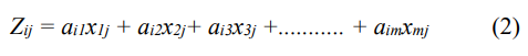
where z represents the score of the component, a denotes the component loading, x stands for the measured value of variables, i denotes the number of the component, j represents the sample number, and m indicates the total number of variables. Based on Juahir et al., (2010), for a better interpretation of principal components (PCs), varimax rotation is recommended to be performed when eigenvalues are above 1.0 [20]. Varimax rotation not only generates new variable groups known as varimax factors (VFs) but also helps identify potential pollution sources. Following previous research, Liu et al., (2003) considered varimax factor (VF) coefficients to be strongly significant if their correlation coefficient is 0.75 or greater, moderately significant if it fell between 0.50 and 0.74, and weakly significant if it ranged from 0.30 to 0.49. Eq. (3) represents this relationship [24]:

In this context, Z represents the measured value of a variable, a denotes the factor loading, f stands for the factor score, e signifies the residual term encompassing errors or other sources of variation, i denotes the sample number, j indicates the variable number, and m represents the total number of factors.

Before conducting further analysis, preliminary assessments are required to ensure that the dataset is sufficient for analysis [25,26]. Additionally, Bartlett's test evaluates whether the variables in a dataset are significantly correlated (p≤0.05), while the KMO test assesses the sampling adequacy, and requires value equal to or greater than 0.5 to confirm that the dataset is sufficient for further analysis.

Artificial Neural Network (ANN) for Air Quality Prediction

Amultilayer perceptron feed-forward neural network was utilized in forecasting the air pollutant index. This model comprises neurons, the basic processing units, organized into three layers: input, hidden, and output, as depicted in Figure 2. The neurons in each layer are interconnected with those in the subsequent layer. The input layer neurons receive input signals, which then pass through weighted connections to the hidden layer for processing. To enhance network performance by finding the best number of hidden nodes and reducing errors, multiple training iterations are conducted with various weight values [27]. This involves employing a backpropagation algorithm for supervised learning, correlating calculated and expected values [27]. Furthermore, the coefficient of determination (R2) and root mean square error (RMSE) justify the performance of the ANN model, with higher R2 and lower RMSE indicating improved prediction accuracy [28]. The corresponding equations are represented as Eq. (4) and Eq. (5).

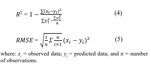
Figure 2: Structure of Multi-Layer Perceptron

Results and Discussion

Descriptive Analysis

Univariate analysis was performed on the historical dataset covering five air quality parameters. Based on the results shown in Table 2, the highest maximum concentrations of PM10, O3, CO, SO2, and NO2 are recorded as 504.250 µg/m , 0.068 ppm, 5.516 ppm, 0.048 ppm, and 0.060 ppm, respectively. The only parameter that shows maximum values greater than RMAQG approved is PM10, while other pollutants showed lower than approved values. However, these values were still permitted due to not exceeding the hazardous level, which is 600 µg/m3 [29]. The highest API recorded is 477, indicating that Peninsular Malaysia has experienced hazardous status (API: 301 and above). Overall mean values for the five air quality parameters in all stations did not exceed the approved level of air pollutant concentration limit based on RMAQG. Moreover, mean values for API also show good status (API:0 – 50).

                                                Table 2: The Results of the Descriptive Analysis of Thirty-Four CAQM Stations

Spatial Clustering of CAQM Stations

Thirty-four (34) air monitoring stations in Peninsular Malaysia were selected and have been classified into three significant clusters by applying HACA. Based on Figure 3, the dendrogram shows three different clusters of monitoring stations, whereby each of them shows similar characteristics within the same cluster. The clusters are known as Low Pollution Cluster (LPC), Moderate Pollution Cluster (MPC), and High Pollution Cluster (HPC). The results proved that HACA can minimize the huge total of active air monitoring stations throughout Peninsular Malaysia, which is meaningful in optimizing the enforcement and monitoring procedures.

Figure 3: Spatial Classification of the Thirty-Four CAQM Stations

Based on the result shown in Table 3, LPC consists of 20 stations, which are Langkawi station (ST4), Alor Setar station (ST5), Sungai Petani station (ST6), Kota Bharu station (ST7), Tanah Merah station (ST8), Balok Baru station (ST14), Indera Mahkota station (ST15), Jerantut station (ST16), Seberang Perai station (ST17), Seberang Jaya station (ST18), Manjung station (ST19), Taiping station (ST20), Pegoh station (ST21), Tasek station (ST22), Tanjung Malim station (ST23), Kangar station (ST24), Kuala Selangor station (ST28), Paka station (ST29), Kuala Terengganu (ST30), and Kemaman (ST31). The average API value for this cluster is 39.16 and the highest value of API recorded was 287, which does not exceed to hazardous level (>300). Based on the findings, almost all air monitoring stations under LPC were categorized as suburban, except Balok Baru station (ST14), Paka station (ST29), and Kemaman station (ST31) were categorized as industrial, while Seberang Jaya station (ST18) and Tasek station (ST22) were categorized as urban. The value of API was consistently at a low level throughout the sampling years (2011-2021) due to the location of the station being isolated from the source of pollutants. Besides, some of the stations are also influenced by meteorological factors, such as wind direction and relative humidity, especially those that receive high volumes of rainfall, such as states in the northern and eastern regions of Peninsular Malaysia. According to Seinfeld and Pandis, (1998); Demuzere et al., (2009), and Ahmad Mohtar et al., (2022) meteorological factors can strongly influence the quality of ambient air through complex interactions between different processes of particulate matter such as transport, emissions, chemical transformation, as well as wet and dry deposition [30-32].

While MPC consists of seven monitoring stations which are Johor Bahru station (ST1), Kota Tinggi station (ST2), Pasir Gudang (ST3), Bukit Rambai station (ST9), Bandaraya Melaka station (ST10), Port Dickson station (ST11), Seremban station (ST13). The highest API record was 477, with an average value of 42.22, and five out of seven stations recorded the highest value API above hazardous level (>300). Based on the findings, all the stations are in the southern region of Peninsular Malaysia. The similarity stations are located near mixed-industrial areas, heavy traffic, and high-density population. In addition, the transboundary could be additional in increased air pollutants [33].

There were seven monitoring stations classified as HPC, which are Nilai station (ST12), Banting station (ST25), Petaling Jaya station (ST26), Shah Alam station (ST27), Batu Muda station (ST32), Cheras station (ST33) and Putrajaya station (ST34). The result has shown that the highest API recorded was at 328 with an average of 50.12. Based on the findings, six out of seven stations were in the central region known as Klang Valley, while Nilai station (ST12) is in the boundary to the central region. This can be seen that the similarity of the stations categorized under this cluster is in surrounded by well-developed areas with high-end industries and commercial, huge development of residential areas to fulfil the demand of high-density population,and heavy traffic congestion associated with the increasing volume of transport on the road. In addition, according to Ahmad et al., (2012), higher air temperature and slower wind speed are significantly associated with experiencing high levels of pollutants due to urban heat phenomena [34].

Table 3: Clusters CAQM Stations Based on the Air Pollutant Index (API)

Discriminant Analysis (DA)

The identification of the most influential parameters for spatial discrimination, as delineated by the clusters generated through HACA, was conducted by employing DA. Three clusters obtained from HACA served as dependent variables, while the five major pollutants served as independent variables. After the three modes of DA were performed, the results revealed with correct assignment rate of 91.87%, signifying that all parameters exhibited significant discrimination with a p-value <0.0001. The matrix of spatial classification performed by DA is presented in Table 4, while Figure 4 illustrates the categorization of monitoring stations into three distinct clusters based on air quality spatial patterns.

Table 4: Spatial Classification by DA

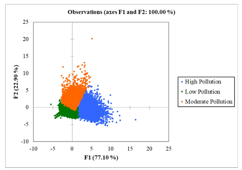
Figure 4: DA Successfully Discriminated Monitoring Stations Based on Air Quality Patterns into Three Different Clusters with 91.87 correct

Identification Source of Variation

A p-value <0.0001 for Bartlett’s test as shown in Table 5 justifies the acceptance of the Ha hypothesis while the result for the KMO test in Table 6 indicates adequacy with a value of 0.614. Therefore, it can be concluded that the variables are correlated, and the samplingis adequate for analysis [26,35].

Table 5: Results of Bartlett’s Sphericity Test

                                                         Table 6: Sampling Adequacy by KMO Measure

Principal component analysis (PCA) was employed to distinguish the patterns of air quality variables and subsequently identify factors associated with the discovered clusters (HPC, MPC, and LPC). The analysis yielded three VFs for HPC and MPC, while four VFs were identified for LPC, all with eigenvalues exceeding 1.0 [36]. Figure 5(i)-(iii) shows the cutoff value retained for further interpretation. The scree plot illustrates the association between the eigenvalues and the number of factors in descending order, explaining the most significant variance in the data. Following the criteria outlined by Liu et al., (2003), factor loadings surpassing 0.75 were deemed significant [24]. Consequently, to pinpoint the most crucial parameters, factor loadings exceeding 0.75 were established as thresholds for further interpretation. Table 7 displays the outcome of factor loadings, with bold figures denoting strong positive loadings (> 0.75). The cumulative variances for the HPC, MPC, and LPC were found to be 65.108 %, 66.279 %, and 60.360 %, respectively. Figure 6(i)-(iii) displays the cumulative variance in the strong loading factors, according to cluster.

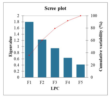
Figure 5(i)-(iii): Scree Plot of PCA Loading

                                                                          Figure 5(i)-(iii): Scree Plot of PCA Loading

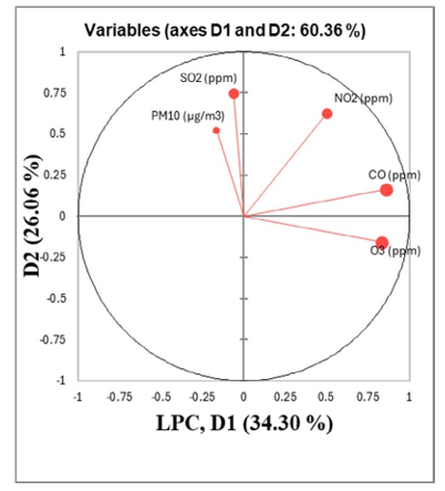
Figure 6(i)-(iii): Factor Loading After Varimax Rotation

High Pollution Cluster (HPC)

In the HPC cluster, VF1, accounting for a total variance of 40.294 %, exhibited strong loadings for NO2 (0.863), and CO (0.803). Conversely, VF2, which represents 24.813 % of the total variance, exhibited a significant loading for O3 (0.881). According to Isiyaka & Azid, (2015), NO2 emissions predominantly arise from industrial activities and motor vehicles [37]. Dominick et al., (2012) have confirmed that NO2 is a product of heavy traffic and manufacturing processes [22]. In Malaysia, approximately 69% of the NO2 released into the air comes from power plants and industrial activities, with motor vehicles accounting for 28% and other sources for the remaining 3% [29]. Elevated levels of CO are linked to inadequate fuel combustion in automobiles, serving as a notable marker of air pollution within the area [38]. Additionally, PM10 levels are linked to road congestion, manufacturing activities, dust from construction sites, and fire burning [39]. Ozone is a byproduct of human activities formed as a secondary pollutant due to complex chemical reactions involving nitrogen oxides (NOX) and volatile organic compounds (VOCs) reacting with sunlight exposure in the presence of heat. Aggressive man-made activities in various socio-economic contexts driven by the demand for industrialization and urban expansion, have increased the emission of NOX and VOCs, consequently leading to ozone formation [40,41].

Moderate Pollution Cluster (MPC)

In the MPC cluster, VF1 accounted for 34.389% of the total variability and exhibited strong loadings on NO2 (0.752) with a negative strong loading on O3 (-0.762). NO2 in the atmosphere originates from both anthropogenic and natural sources, including vehicle exhaust, industrial activities, soil microbial processes, and lightning. Nevertheless, the elevated NO2 levels observed in urban settings predominantly stem from motor vehicles and industrial emissions [42]. O3 showed negative values, demonstrating an inverse relationship among the variables. Known as a secondary pollutant, ozone is produced through photochemical reactions of NOX and VOCs in the presence of heat and sunlight. Hence, the value of O3 is likely affected by this process. Due to the elevated emission of NOX from traffic sources, the concentration of O3 diminishes as it disperses during the oxidation of NOX [43]. Consequently, this process results in a negative impact on O3 levels. Concurrently, VF2 contributed 31.890% of the total variance and displayed a strong loading of PM10 (0.888). According to Zakaria et al. (2018) and Sahak et al. (2022), PM10 is produced by point sources such as power generation, industrial operations, construction sites, and automobile emissions [43,44]. PM10 is primarily emitted from heavy construction associated with urban development, as well as from the resuspension of soil and road dust [37].

Low Pollution Cluster (LPC)

VF1 accounted for 34.304% of the total variability, displaying strong loadings on O3 (0.834) and CO (0.858). The high concentration of O3 is largely dependent on the presence of its precursors (NOX, CO, and VOCs), as it is a secondary pollutant. NOX and VOCs stem from manufacturing activities and vehicular emissions (Molina et al., 2019), while CO emanates from the incomplete combustion of fuel in vehicles, manufacturing factories, incinerators, and open-air burning activities [29]. VF2, which represents 26.056% of the total variance, exhibited a strong loading on SO₂ (0.757). The heightened levels of SO2 detected in this grouping are probably connected to chemical constituents originating from fossil fuel burning, notably from power plants, industrial facilities, and vehicle emissions [45-47].

Air Quality Prediction Using ANN

Predicting the Spatial Distribution

Analysis was performed with ten network structures to test the MLP-FF-ANN model for predicting the spatial distribution of air quality variables in the three significant clusters (HPC, MPC, and LPC) in Peninsular Malaysia. Table 8 shows that the MLP-ANN model successfully discriminated spatial patterns into HPC, MPC, and LPC accordingly. The optimum performance of the model was recorded at node eleven with the highest R2=0.9472, RMSE=0.1854 for training and R2=0.9492, RMSE=0.1826 for testing, indicating a very strong correlation (Schober et al., 2018). Further result analysis can also be seen in Table 9, where the MLP-FF-ANN model successfully discriminated the air pollution datasets based on clusters (HPC, MPC, LPC) with an average correct classification rate of 94.30 %, outperforming DA analysis with an average correct classification rate of 91.87 %. Figure 7 shows the performance of the receiver operating characteristic (ROC) based on the area under the ROC curve (AUC). Referring to Bekkar et al. (2013), and Deary & Griffiths (2021), a value higher than 0.9 indicates excellence [48,49]. Therefore, this analysis demonstrates that the MLP-FF-ANN model is an excellent classifier parameter, with the values for HPC, MPC, and LPC being 0.9923, 0.9913, and 0.9937 respectively.

Table 8: Prediction Performance of Spatial Pattern Recognition Using MLP-FF-ANN

                                                 Table 9: Comparison Results of Classification Matrix by (i) ANN and (ii) DA

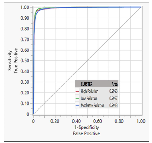
Figure 7: Receiver Operating Characteristics (ROC) for Spatial Distribution of Air Quality Parameters in Peninsular Malaysia

Predicting Air Pollutant Index

The API was forecasted using the MLP-FF-ANN model, in which underwent ten iterations to train the network and achieve a precise approximation of any non-linear function. As depicted in Table 10, the MLP-FF-ANN model demonstrated optimal predictive performance during training at node nine, yielding the highest R² value of 0.7774 and the lowest RMSE value of 9.9048. Subsequently, the model's network was validated, resulting in R2 and RMSE values of 0.7744 and 9.8548, respectively. The scatter plot diagram in Figure 8 illustrates the ANN's ability to forecast API levels. In this analysis, five major pollutants were used as input parameters. According to Rumsey (2011), the value of R2 in this finding is categorized as significant with a strong correlation [50]. This means that the prediction model explains around 77 % of the variation well, as compared to the actual API values by the DOE.

                                                                  Table 10: Prediction Performance of API Using MLP-FF-ANN

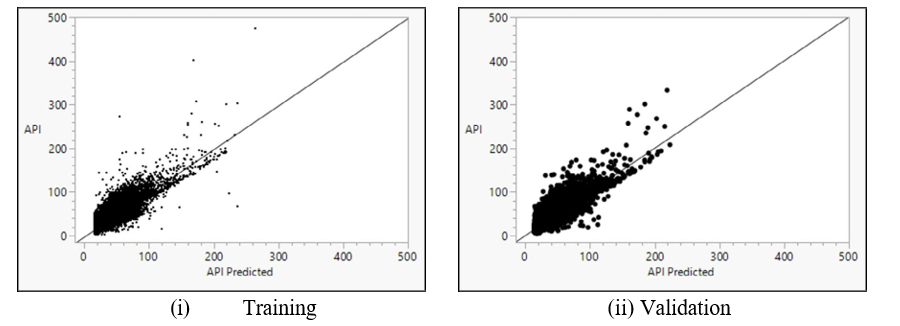
 Figure 8: Scatter Plot of API Predicted vs Actual API

Conclusion

The findings of this research study demonstrate that environmetric techniques are reliable tools for assessing air quality patterns. HACA has simplified the mass data collection from thirty-four CQAM stations into three significant clusters labeled HPC, MPC, and LPC, which could potentially serve as evidence for considering a reduction in monitoring stations. Results from DA, utilizing standard, forward, and backward stepwise modes, exhibited a high accuracy rate of cluster assignation, with 91.87 % correct, indicating significant discrimination among the five parameters (PM10, SO2, NO2, CO, and O3) in all modes with a p-value <0.0001. This underscores the importance of closely monitoring all five air quality parameters. PCA identified two varifactors (VFs) in all clusters assigned by HACA, with cumulative variances of HPC (65.108 %), MPC (66.279 %), and LPC (60.360 %). The major pollutants were identified in each cluster, whereby NO2, CO, and O3 showed strong positive loadings in HPC, NO2 and PM10 presented strong positive loadings, while O3 showed an inverse relationship in MPC. Three strong positive loadings were obtained from SO2, O3, and CO in LPC. The presence of pollutants varies in each cluster and is associated with anthropogenic and natural sources in the locality. By gaining this evidence, monitoring and enforcement could be more specific and strategized.

Utilizing the MLP-FF-artificial neural network in this assessment offers an effective method for monitoring air quality. The MLP-FF-ANN model demonstrated a spatial classification accuracy of 94.30% for CAQM, surpassing the performance of discriminant analysis (DA). Thus, it is suggested that the hybrid method provides precise and accurate results for classifying air quality status. By incorporating the results of PCA, five major pollutants were utilized in performing MLP-FF-ANN to predict API readings. The results obtained were R2=0.7774 and RMSE=9.9048, indicating a significant and strong correlation. These findings support the guidelines of the DOE to monitor these five major pollutants in order to determine API values. Therefore, with the combination of these two findings, PCA and ANN, valuable insights are offered for refining air quality monitoring workflows, thereby facilitating informed decision- making and effective control strategies to mitigate adverse effects while optimizing resource allocation.

Acknowledgments

The author extends sincere appreciation to the Department of Environment of Malaysia and East Coast Environmental Research Institute (ESERI), Universiti Sultan Zainal Abidin, Malaysia, for the invaluable guidance in completing this research project.

References

1. Chen, H., Deng, G., & Liu, Y. (2022). Monitoring the influence of industrialization and urbanization on spatiotemporal variations of AQI and PM2. 5 in three provinces, China. Atmosphere, 13(9), 1377.
2. Zhang, G., Ren, Y., Yu, Y., & Zhang, L. (2022). The impact of air pollution on individual subjective well-being: evidence from China. Journal of Cleaner Production, 336, 130413.
3. Hadley, M. B., Vedanthan, R., & Fuster, V. (2018). Air pollution and cardiovascular disease: a window of opportunity. Nature Reviews Cardiology, 15(4), 193-194.
4. Tran, H. M., Tsai, F. J., Lee, Y. L., Chang, J. H., Chang, L.T., Chang, T. Y., ... & Chuang, H. C. (2023). The impact of air pollution on respiratory diseases in an era of climate change: A review of the current evidence. Science of the Total Environment, 166340.
5. Ab Manan, N., Aizuddin, A. N., & Hod, R. (2018). Effect of air pollution and hospital admission: a systematic review. Annals of global health, 84(4), 670.
6. Abed Al Ahad, M., Sullivan, F., Demšar, U., Melhem, M., & Kulu, H. (2020). The effect of air-pollution and weather exposure on mortality and hospital admission and implications for further research: A systematic scoping review. PloS one, 15(10), e0241415.
7. Abed Al Ahad, M. (2024). Air pollution reduces the individuals’ life satisfaction through health impairment. Applied Research in Quality of Life, 1-25.
8. Druzhinin, P. V., Shkiperova, G. T., Potasheva, O. V., & Zimin, D. A. (2020). The Assessment of the Impact of the Economy's Development on Air Pollution. Ekonomicheskie i Sotsialnye Peremeny, 13(2), 125-142.
9. de Araújo Leal, R., da Silva, T. A., Mergulhão, T. J. C., Monteiro, E. C. B., & Takaki, G. M. C. (2023). Factors and consequences of acid rain incidence. Seven Editora.
10. Twagirayezu, G., Nizeyimana, J. C., Irumva, O., Ntakiyimana, C., Uwimpaye, F., Nyirandayisabye, R., ... & Hakuzweyezu, T. (2023). A Critical Review of Acid Rain: Causes, Effects, and Mitigation Measures.
11. Siriopoulos, C., Samitas, A., Dimitropoulos, V., Boura, A., & AlBlooshi, D. M. (2021). Health economics of air pollution. In Pollution Assessment for Sustainable Practices in Applied Sciences and Engineering (pp. 639- 679). Butterworth-Heinemann.
12. Jaafar, H., Razi, N. A., Azzeri, A., Isahak, M., & Dahlui,M. (2018). A systematic review of financial implications of air pollution on health in Asia. Environmental Science and Pollution Research, 25, 30009-30020.
13. Liu, Y. M., & Ao, C. K. (2021). Effect of air pollution on health care expenditure: Evidence from respiratory diseases. Health Economics, 30(4), 858-875.
14. Lee, Y., Yang, J., Lim, Y., & Kim, C. (2021). Economic damage cost of premature death due to fine particulate matter in Seoul, Korea. Environmental Science and Pollution esearch, 28(37), 51702-51713.
15. Thangavel, P., Kim, K. Y., Park, D., & Lee, Y. C. (2023). Evaluation of Health Economic Loss Due to Particulate Matter Pollution in the Seoul Subway, South Korea. Toxics, 11(2), 113.
16. Sofia, D., Gioiella, F., Lotrecchiano, N., & Giuliano, A. (2020). Mitigation strategies for reducing air pollution. Environmental Science and Pollution Research, 27(16), 19226-19235.
17. Abbass, K., Qasim, M. Z., Song, H., Murshed, M., Mahmood, H., & Younis, I. (2022). A review of the global climate change impacts, adaptation, and sustainable mitigation measures. Environmental Science and Pollution Research, 29(28), 42539-42559.
18. Isiyaka, H. A., & Azid, A. (2015). Air quality pattern assessment in Malaysia using multivariate techniques. Malaysian Journal of Analytical Sciences, 19(5), 966-978.
19. Rahman, E. A., Hamzah, F. M., Latif, M. T., & Dominick, D. (2022). Assessment of PM2. 5 Patterns in Malaysia Using the Clustering Method. Aerosol and Air Quality Research, 22(1), 210161.
20. Juahir, H., Zain, S. M., Aris, A. Z., Yusoff, M. K., & Mokhtar,M. B. (2010). Spatial assessment of Langat river water quality using chemometrics. Journal of Environmental Monitoring, 12(1), 287-295.
21. Pati, S., Dash, M. K., Mukherjee, C. K., Dash, B., & Pokhrel, S. (2014). Assessment of water quality using multivariate statistical techniques in the coastal region of Visakhapatnam, India. Environmental monitoring and assessment, 186, 6385-6402.
22. Dominick, D., Juahir, H., Latif, M. T., Zain, S. M., & Aris,A. Z. (2012). Spatial assessment of air quality patterns in Malaysia using multivariate analysis. Atmospheric environment, 60, 172-181.
23. Eder, B., Bash, J., Foley, K., & Pleim, J. (2014). Incorporating principal component analysis into air quality model evaluation. Atmospheric Environment, 82, 307-315.
24. Liu, C. W., Lin, K. H., & Kuo, Y. M. (2003). Application of factor analysis in the assessment of groundwater quality in a blackfoot disease area in Taiwan. Science of the total environment, 313(1-3), 77-89.
25. Tabachnick, B. G., Fidell, L. S., & Ullman, J. B. (2013). Using multivariate statistics (Vol. 6, pp. 497-516). Boston, MA: pearsonhttps://www.pearsonhighered.com/assets/ preface/0/1/3/4/0134790545.pdf.
26. Shihab, A. S. (2022). Identification of Air Pollution Sources and Temporal Assessment of Air Quality at a Sector in Mosul City Using Principal Component Analysis. Polish Journal of Environmental Studies, 31(3).
27. Arhami, M., Kamali, N., & Rajabi, M. M. (2013). Predicting hourly air pollutant levels using artificial neural networks coupled with uncertainty analysis by Monte Carlo simulations. Environmental Science and Pollution Research, 20, 4777-4789.
28. Sarkar, A., & Kumar, R. (2012). Artificial neural networks for event based rainfall-runoff modeling. Journal of Water Resource and Protection, 4(10), 891.
29. Ab Malek, H., Jalaluddin, N. N. N., Hasan, S. N. S., Hassni, U. A., & Ab Malek, I. (2021). AIR POLLUTION ASSESSMENT IN SOUTHERN PENINSULAR MALAYSIA USING ENVIRONMETRIC ANALYSIS.
30. Malaysian Journal of Analytical Sciences, 25(5), 821-830.Seinfeld, J. H., & Pandis, S. N. (2016). Atmosphericchemistry and physics: from air pollution to climate change.John Wiley & Sons.
31. Demuzere, M., Trigo, R. M., Vila-Guerau de Arellano, J., & Van Lipzig, N. P. M. (2009). The impact of weather and atmospheric circulation on O 3 and PM 10 levels at a rural mid-latitude site. Atmospheric Chemistry and Physics, 9(8), 2695-2714.
32. Mohtar, A. A. A., Latif, M. T., Dominick, D., Ooi, M. C.G., Azhari, A., Baharudin, N. H., ... & Juneng, L. (2022). Spatiotemporal variations of particulate matter and their association with criteria pollutants and meteorology in Malaysia. Aerosol and Air Quality Research, 22(9), 220124.
33. Sentian, J., Herman, F., Yih, C. Y., & Wui, J. C. H. (2019). Long-term air pollution trend analysis in Malaysia. International Journal of Environmental Impacts, 2(4), 309- 324.
34. Ahmad, M. N., Sidek, L. M., Selamat, A., & Abidin,R. Z. (2012, November). THE RELATIONSHIP OF LOCALIZED RAINFALL VERSUS URBAN HEAT ISLAND (UHI) PARAMETERS AND AIR POLLUTION.In International Conference On Water Resource.
35. Bartlett, M. S. (1954). A note on the multiplying factors for various χ 2 approximations. Journal of the Royal Statistical Society. Series B (Methodological), 296-298.
36. Kim, J. O., & Mueller, C. W. (1978). Introduction to factor analysis: What it is and how to do it (No. 13). Sage.
37. Isiyaka, H. A., & Azid, A. (2015). Air quality pattern assessment in Malaysia using multivariate techniques. Malaysian Journal of Analytical Sciences, 19(5), 966-978.
38. Angatha, R. K., & Mehar, A. (2020). Impact of traffic on carbon monoxide concentrations near urban road mid- blocks. Journal of The Institution of Engineers (India): Series A, 101, 713-722.
39. Rosman, P. S., Samah, M. A., & Yunus, K. (2019). A research on concentration and distribution of airborne particulate matter in Kuantan city. Int. J. Recent Technol. Eng, 8(2S3), 288-292.
40. An, Z., Huang, R. J., Zhang, R., Tie, X., Li, G., Cao, J., ...& Ji, Y. (2019). Severe haze in northern China: A synergy of anthropogenic emissions and atmospheric processes. Proceedings of the National Academy of Sciences, 116(18), 8657-8666.
41. Tian, Y., Wang, Y., Han, Y., Che, H., Qi, X., Xu, Y., ... & Wei,C. (2023). Spatiotemporal characteristics of ozone pollution and resultant increased human health risks in central China. Atmosphere, 14(10), 1591.
42. Hu, M., Chen, Y., Yuan, D., Yu, R., Lu, X., Fung, J. C.,... & Lau, A. K. (2022). Estimation and spatiotemporal analysis of NO2 pollution in East Asia during 2001–2016. Journal of Geophysical Research: Atmospheres, 127(2), e2021JD035129.
43. Zakri, N. L., Saudi, A. S. M., Juahir, H., Toriman, M. E., Abu,I. F., Mahmud, M. M., & Khan, M. F. (2018). Identification source of variation on regional impact of air quality pattern   using chemometric techniques in Kuching, Sarawak. Int J Eng Technol, 7(49), 10-14419.
44. Sahak, N., Asmat, A., & Yahaya, N. Z. (2022). Spatio- Temporal Air Pollutant Characterization for Urban Areas. Journal of Geoscience and Environment Protection, 10(1), 218-237.
45. Wei, X., Liu, Q., Lam, K. S., & Wang, T. (2012). Impact of precursor levels and global warming on peak ozone concentration in the Pearl River Delta Region of China. Advances in Atmospheric Sciences, 29, 635-645.
46. Mutalib, S. N. S. A., Juahir, H., Azid, A., Sharif, S. M., Latif,M. T., Aris, A. Z., ... & Dominick, D. (2013). Spatial and temporal air quality pattern recognition using environmetric techniques: A case study in Malaysia. Environmental Science: Processes & Impacts, 15(9), 1717-1728.
47. Mohtar, A. A. A., Latif, M. T., Baharudin, N. H., Ahamad, F., Chung, J. X., Othman, M., & Juneng, L. (2018). Variation of major air pollutants in different seasonal conditions in an urban environment in Malaysia. Geoscience Letters, 5(1), 1-13.
48. Bekkar, M., Djemaa, H. K., & Alitouche, T. A. (2013). Evaluation measures for models assessment over imbalanced data sets. J Inf Eng Appl, 3(10).
49. Deary, M. E., & Griffiths, S. D. (2021). A novel approach to the development of 1�hour threshold concentrations for exposure to particulate matter during episodic air pollution events. Journal of Hazardous Materials, 418, 126334.
50. Rumsey, D. J. (2011). Statistics For Dummies. John Wiley & Sons.
51. Department of Environment (DOE) (2018) Malaysia Environmental Quality Report 2018. Department of Environment, Putrajaya, Malaysia. (n.d.). In
52. Environmental Data Center. (n.d.). Department of Environment. Retrieved March 23, 2024.
53. Lau, J., Hung, W. T., & Cheung, C. S. (2009). Interpretation of air quality in relation to monitoring station's surroundings. Atmospheric Environment, 43(4), 769-777.
54. Love, D., Hallbauer, D., Amos, A., & Hranova, R. (2004). Factor analysis as a tool in groundwater quality management: two southern African case studies. Physics and Chemistry of the Earth, Parts A/B/C, 29(15-18), 1135-1143.
55. Molina, L. T., Velasco, E., Retama, A., & Zavala, M. (2019). Experience from integrated air quality management in the Mexico City Metropolitan Area and Singapore. Atmosphere, 10(9), 512.
56. Schober, P., Boer, C., & Schwarte, L. A. (2018). Correlation coefficients: appropriate use and interpretation. Anesthesia & analgesia, 126(5), 1763-1768.
57. Zakaria, U. A., Saudi, A. S. M., Abu, I. F., Azid, A., Balakrishnan, A., Amin, N. A., & Rizman, Z. I. (2017). The assessment of ambient air pollution pattern in Shah Alam, Selangor, Malaysia. Journal of Fundamental and Applied Sciences, 9(4S), 772-788.