Introduction

The composition and thickness of the crust are important to com- prehend the continent's creation and evolution. Although surface geochemical study has helped us understand the upper crust better, we still don't know much about the intermediate and lower crust. According to reports, seismic wave velocity in the lower crust, for example, varies significantly (Vp 6.5–7.1 km s1) and may be a sign of highly distinct lithologies and, consequently, the evo- lutionary process. In contrast to earlier theories propose a lower crust that is more felsic and roughly three times more radiogenic [1-3]. This has consequences for our comprehension of the thermal state of the lithosphere and emphasises the need for an accurate representation of the thickness and seismic wave velocity of dif- ferent segments of the crust. Understanding the evolution of the continental crust requires an understanding of how an andesitic to dacitic crust evolved although most mantle-derived magma has a basaltic nature [4]. Mapping the variety or similarity of crustal composition at different geological depths is therefore necessary.

As important, is figuring out what kind of first-order compositional discontinuity Moho is when seismic wave velocity rapidly increas- es from a typical felsic-mafic crust value with Vp > 7.8 km s1 and Vs > 4.3 km s1 reflecting ultramafic peridotites [5,6]. According to this scenario, there will be a thin, one to two kilometer wide tran- sition at the Moho state that the Moho and the crust-mantle border do not always line up [7]. According to an analysis of crustal scale wide angle pro-files conducted globally, Moho may, in some cases, represent the top of lower crustal eclogites connected to previous orogenies [8,9]. Mafic rocks (pyroxene–garnet granulite facies) change into eclogite at a depth of roughly 50–70 km beneath the previously enlarged crust. Ultimately, the combined processes of erosion and isostatic relaxation push the original root down to a depth of 30 to 50 kilometers.

There are such well-preserved crustal roots with local lengths of 60 km mapped in cratonic regions of Europe [4,10-12]. Because eclogite and peridotite have similar seismic wave velocities, fur- ther restrictions like as anisotropy and density mapping make it challenging to distinguish between the two A largely eclogitic low- er crust may have a density of roughly 3.0 g cc1, which is compa- rable to unplanted material. Typically, a lower crust eclogite has a density of 3.5 g cc1. Here, we also investigate Moho's topography, specifically if it is rocky or flat, in addition to its crustal makeup. It's mysterious in either scenario. We are unable to fully compre- hend, for example, the mechanism generating a nearly flat Moho or the mechanism by which adjacent blocks with wildly disparate Moho depths survive throughout time [13]. Understanding the physicochemical characteristics of the crust and the structure of the crust-mantle boundary is essential for simulating the processes that led to the development of the continental crust, its relationship with surface geology, and the crust's persistence across billions of years. We provide the Rayleigh-wave group velocity data and joint inversion of tele-seismic receiver functions from 50 broad-band seismographs that uniformly sampled the region to determine the shear wave velocity of the crust in the Dharwar Craton (5–70 s) in order to address some of the previously mentioned questions. Additional measurements for the 40-70-second time window are derived from Acton et al. and the dispersion data for the 5-28-sec- ond time range are generated using ambient noise.

Materials and Methods

Geological Structure of the Dharwar Craton

The Dharwar craton, located in southern India, is a remnant of the Archean continental plate that has a continuously exposed crustal section ranging from greenstone basins and low-grade gneisses to granulite’s . There are three main lithological units that make up this region: the K-rich granitoids (such as N-S trending Close pet Granite (CG)) with an age of 2.5-2.6 Ga; the volcano-sedimentary greenstone belt with two distinct ages (3.3-3.1 Ga and 3.2-2.7 Ga; and the peninsular gneisses with a composition of tonalite, trondh- jemite, and granodiorite (TTG) that range in age from 3.36 to 2.7 Ga Taylor et al., Meen et al, and the peninsular gneisses with a composition of tonalite, trondhjemite, and granodiorite (TTG) that range in age from 3.36 to 2.7 Ga [14]. Chitra Durga Schist Belt (CSB) divides the craton into the West Dharwar Craton (WDC) and East Dharwar Craton (EDC) based on ages and lithologies [15]. Greenstone and gneisses from the 3.3–3.0 Ga era make up the WDC, along with a few isolated areas of newer granite. While the 3.0-2.7 Ga Dharwar Basins 11 (Dhar wars) make up the north- ern portion of the WDC, the 3.36 Ga greenstone belts (red dashed ellipse in Figure 1 ) form the south-central portion of the WDC and contain some of the oldest rocks of the Indian continents. A greater degree of metamorphism is seen in the WDC, which exposes rocks with 500ºC and 3-5 Kb (greenschist facies) in the north (at 15ºN) and 8 Kb and 800ºC (granulite facies) in the south (at 13ºN). This indicates tectonic upliftment and erosion extending from 4 km in the north to around 12 km in the south. The Proterozoic Kaladgi Basin (KB) and Bhima Basin (BB) as well as the Deccan Volcanic Province (DVP), a vast region of Cretaceous flood basalts, enclose the WDC in the north and mask the northern boundaries of the bur- ied craton. The late Archean (2.7–2.5 Ga) calc-alkaline complex of juvenile and anatectic granites, granodiorites, and diorites, also known as Dharwar batholiths, dominates the EDC [11].

The EDC is shoved into the Eastern Ghats Granulite topography (Eastern Ghats) and the massive crescent-shaped Proterozoic Cud- dapah Basin (CB). A notable geological formation with many min- eral occurrences is the CB. The basin is block faulted and mostly evolved approximately 1700 Ma. Numerous phases of igneous activity have an impact on its southern region [16]. The southern sediments have undergone more metamorphosis than the northern ones. Given its positive Bouguer anomaly and implied thrust con- tact with the CB, the Eastern Ghats is the most easterly situated geological terrain. Every rock in the Eastern Ghats is an igneous or metamorphosed deposit (mostly free rocks of pyroxene and khon- dalite). The age of these rocks ranges from 1615 to 995 Ma. The Western Ghats is the westernmost geological block in the research area. It is a ~50 km broad, topographically high (~1.2 km), paral- lel to the coast belt that is associated with the ~80 Ma separation of Madagascar from India [17]. The craton gradually gives way to the Southern Granulite Terrain (SGT), a region commonly re- ferred to the Archean metamorphic terrain (2.6 Ga). A dispersed orthopyroxene is grade divides the two terrains. The well-known Moyar shear zone (MSZ) and Bhavani shear zone (BSZ) split the granulite’s, and in the western sector, they reach to heights of up to 2300 meters, forming the Nigiri Hills. Beyond the Noyil-Kaveri shear zone (NKSZ) (Figure 1), the high-grade granulite’s connect to the metamorphic terrains of Pan African orogeny, which span the southern tip of the Indian Peninsula and have a shared history with terranes that stretch from East Africa to Antarctica, such as the Tanzanian shield, Madagaskar, and Sri Lanka. These terrains date back approximately 600 million years.

The Deccan Volcanic Province (DVP), the Southern Granulite Ter- rain (SGT), the East and West Dharwar Craton (WDC), and Chitra Durga Schist Belt (CSB), Cuddapah Basin (CB), Kaladgi Basin (KB), Bhima Basin (BB), Moyar Shear Zone (MSZ), Bhavani Shear Zone (BSZ), and Noyil-Kavery Shear Zone (NKSZ). Black dashed lines indicate shears. The black and red dashed ellipses, re- spectively, indicate the Dharwar Schist and Greenstone belt, which are located to the north and south of WDC.

Studies on Geophysics in the Dharwar Craton

Studies on Seismic Activity

Currently available seismic wave velocity, surface wave and tele seismic waveforms (receiver function) from a few broadband seis- mograph locations, and modelling of wide angle reflection and re- fraction measurements along a profile form the basis of much of our understanding of the nature of the crust beneath the Dharwar craton. Kaila and Krishna modelled an upper crust with P wave velocity of 6.4 km/s, lower crust velocity of 6.7 km/s, and Moho depth varied from 34 km in the east to 41 km in the west using seismic reflection/refraction data from Kavali-Udipi profile over the WDC/EDC [17]. According to Mitra et al. the inversion of Rayleigh wave phase velocity in the EDC indicates an average crustal thickness of 35 km, with a layer 12 km thick (Vs = 3.66 km/s) covering a 23 km thick (Vs = 3.81 km/s) lower crust.

The Gravitational Field and Topography

Even though the Dharwar craton is primarily Archean terrain, there is a lot of diversity in the pattern of height (Figure 2 a). The geography in the EDC and WDC is flat, ranging from about 400 to 800 metres. On the other hand, the southern granulite’s have a high height with topography varying from around 1000 to 2700 metres. The higher elevation of Western and Eastern Ghats (1200 and 700 m, respectively) dramatically disrupts the typical elevation of the coastal plains on either side of the Dharwar craton that adjoins the sea. Figure 2 (b) depicts the Bouguer gravity anomaly map of the Dharwar craton (NGRI), which demonstrates notable fluctuations in both anomaly pattern and magnitude. Anomaly varies from -70 to -130 mGal over the craton. Southern WDC and SGT are two of the areas with noticeable low gravity anomalies (~-100 gal). It is well known that the crust on these terrains is thicker [11]. A gravity value of about -20 mGal is indicative of the Eastern Ghats. The reason behind this is either high-density intrusive or crustal weakening [11].

Figure 2: Map of the Dharwar Craton's Topography, (a) Thick Dark Lines Indicate Major Tectonic Structures. (b) Map of the Dharwar Craton's Bouguer Gravity Anomalies (after Ngri, 1978). Plotting and Annotation of Contours Occur at Intervals of

Broadband Seismological Experiment at Dharwar

This thesis makes use of data from fifty broadband seismograph locations (Table 1) established and maintained by the Geophysi- cal Field Research Group, Hyderabad, in the Dharwar craton. The remaining 15 sites were a part of an earlier experiment that ran from June 1999 to June 2012, whereas the majority of these sta- tions—35—were in operation from 2019 to 2021 [12]. These sta- tions have GURALP manufacture CMG3T/3ESP sensors, which are sensitive to ground vibration in the frequency range of 120/40 s to 50 Hz, along with a REFTEK data requisition system. We recorded the earthquake waveforms continuously at a rate of 50 samples per second.

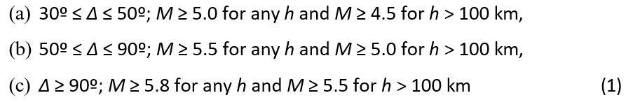
Data are downloaded to compact discs and external hard drives after every visit to seismic stations (CD). Data are retrieved onto the system and transformed into a legible format known as seismo- grams using pre-established earthquake criteria. The preliminary determination of earthquakes, or PDEs, from the US Geological Survey (USGS) are used to choose earthquakes. The selection cri- teria for the occurrences comprised of the following: magnitude (M), focal depth (h) in kilometers, and epicentral distance (â??) in degrees.

                         Table 1: Location of the Stations of the Dharwar Craton Along with the Operational Period

A Mathematical Method for Estimating Receiver Func- tions

A well-known seismological method for obtaining data on the in- terior structure of the Earth, particularly the layer thickness and seismic wave velocity, is the receiver function (RF) methodology. The reaction of the Earth structure close to the receiver is includ- ed in this time series, which was calculated using three-component seismograms [4]. The mechanism relies on the fact that near vertical seismic waves (P and S) arrive at the layer border, where velocity contrast is present, and transform into one another. This pertains to the transformation of a tele seismic P wave into a S wave. P and S waves, two types of seismic body waves, go through the Earth's interior at the following velocities:

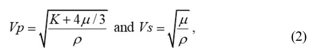
Where ρ is the medium's density, K is the bulk modulus, and μ is the shear modulus. Seismic waves are either reflected or refracted in accordance with Snell's law when they encounter an interface between two media. According to Langston a tele seismic P wave can produce a three-component seismic waveform that records D in the time domain [18].

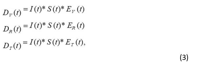
where * denotes the convolution operator, I(t) is the instrument's impulse response, S(t) is the seismic source function, E(t) is the local earth structure's impulse response, and subscripts V, R, and T stand for the vertical, radial, and tangential components, respec- tively. Within the frequency range, one may possess

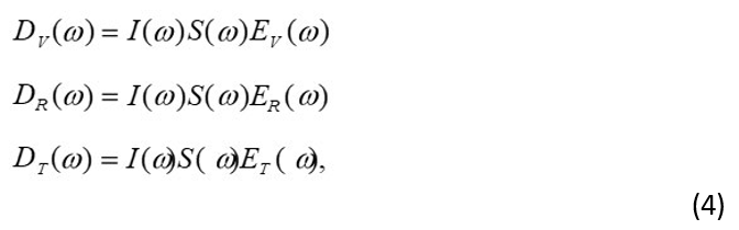
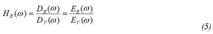
Where DV(ω) represents DV(t) ext.’s Fourier Transform. Simple division of the foregoing equation will remove the source and instru- ment terms, giving rise to the radial receiver function, or HR(ω).

According to Langston for a steeply incident P wave, the vertical component of ground motion consists of a significant direct arrival followed by only small arrivals from phase conversions and crust- al reverberations [18]. Consequently, suggested that EV(t) = δ(t), where δ(t) is the Dirac delta function. The term "source equalization scheme" describes this. Consequently, HR(ω) ≈ ER(ω). Thus, the tangential receiver function, HT(ω) ≈ ET(ω), is approximately equivalent to the radial impulse response of the Earth structure, as is the case with the radial receiver function.

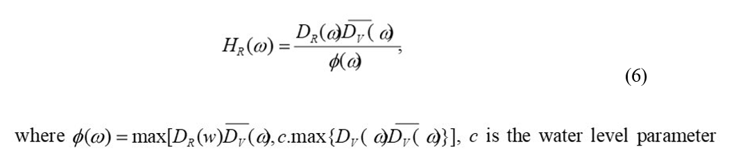
The seismogram with a high signal-to-noise ratio can use the above formula. The technique is unstable when noise is present, just like in real data. As a result, equation was changed in accor- dance with Clayton and Wiggins. The change entails setting the water level, or minimum permissible amplitude level, for the verti- cal component's amplitude spectrum. By decreasing in magnitude, the water level stabilizes the de convolution of the trough in the vertical component spectrum to prevent division when applying equation below by extremely small values. Rewriting equation be-low as follows:

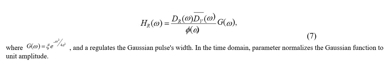
In order to eliminate high frequency noise from the final results, this estimate is typically smoothed using a Gaussian function. Thus, at last, one can acquire

Shear Velocity Structure of Crust Beneath the Dharwar Craton

Data Analysis

It has been possible to analyses the nature of Moho and the seismic wave velocity in the crust at different depths beneath each individual seismograph location in the Dharwar craton for the first time thanks to an adequate coverage of broadband seismic stations (50 nos.) (Figure 3).

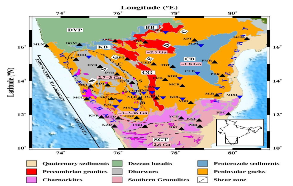
Figure 3: Shows the Location of Seismic Stations Utilized in the Study together with a Tectonic Map of the Dharwar Craton. Blue Inverted Triangles Date from 1998 to 2012, Whereas Black Triangles Show Seismographs that were in Use from 2019 to 2021

The receiver functions are calculated using the time domain iter- ative deconvolution approach, as was previously discussed [19]. We use earthquakes with a magnitude greater than 5.5 and an epi- central distance ranging from 30 to 95 degrees. The majority of earthquakes occur in north to south-east directions, resulting in an azimuthal tilt in the data available for stations due to geographical limitations. Figure 4, which depicts the distribution of earthquakes for a typical station AMT, illustrates this.

Figure 4 : Using Data from Station Amt (Black Triangle), the Epicenter Locations of Earthquakes with a Magnitude Greater Than 5.5 are Shown as Red Circles

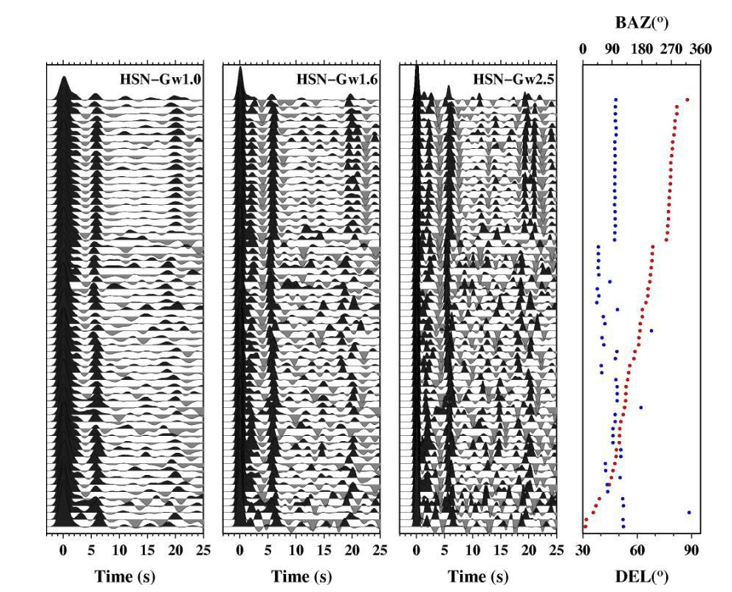
Figure 5: Shows The Receiver Functions for the Various Gaussian Widths (GW) of 1.0, 1.6, And 2.5 at the HSN Station (in the WDC). Plotted in the left Panels for Each Receiver Function, the Extreme Right Panel Displays the Values for the Back Azimuth (Blue Circle) and Epicentral Distance (Red Circle)

During the deconvolution process, a Gaussian filter with widths (Gw) of 1.0, 1.6, and 2.5 was employed to determine the best fre- quency range for computing the receiver function. Figure 6 dis- plays the receiver functions for station HSN, which is located in the southern WDC, in relation to the three Gaussian widths. Be- cause the receiver functions for Gw1.0 are smoother and limit the identification of intra-crustal layers, Gw1.6 is favored over Gw2.5, which has more noise.

Out of the initial set of about 4000 receiver functions, over 2500 receiver functions with a waveform fit of more than 80% were chosen for in-depth investigation. Figures A.1 through A.7 show the receiver functions plotted with back azimuth for each station. Subsequent analysis of the receiver function across all stations in- dicates the presence of three distinct categories for seismograph locations, which indicate the underlying geological complexity: A- with distinct P-to-S conversion (Ps) and multiples (PpPms, PpSms); B- with distinct Ps and PpPms (or PpSms); and C- with distinct Ps only. Figure 7 displays an example of these three groups of receiver functions from various seismograph locations. Figure 7 displays the distribution of quality seismograph locations in the Dharwar Craton based on these criteria.

Figure 6: Shows the Quality of the Receiver Functions (A, B, Or C) at the Three Stations that Serve as Examples: GBA, APT, and NLR. Clear P-To-S Conversion (Ps) and Multiples (PpPms, PpSms) are Present in Quality A; Ps and PpPms (Or PpSms) are Present in Quality B; and Ps Is the Sole Clear P.

Figure 7: Receiver Function Quality as Calculated at Each Study Station in the Area. the Positions of the Three Profiles (AA/, BB/, and CC/) that the Migrated Receiver Functions are Plotted Along are Indicated by Thick lines in Figure 8

Moho Depth and Average Vp/Vs Ratio Estimation

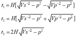
Zhu and Kanamori developed the H-Vp/Vs stacking technique, which uses the knowledge that known functions of Moho depth (H), Vp/Vs ratio, and average Vp in the crust determine arrival times and amplitude of specific Moho converted phases and multi- ples appearing on radial receiver functions, to obtain Moho depth (H) and average Vp/Vs ratio (or Poisson’s ratio σ) [13]. Since travel times are substantially less sensitive to Vp than to Vs when employed for crustal receiver function analysis an average Vp for the entire crust is taken from previously collected seismic source investigations in the area [3,20,21]. The receiver function ampli- tude, defined as S(H, Vp/Vs), should be at its maximum for a near- true combination of H and Vp/Vs ratio value during the comput- ed times of expected arrivals of Ps, PpPms, and PpSms+PsPms phases.

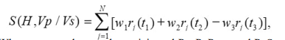
Where t₁, t₂, and t₃ are the anticipated Ps, PpPms, and PpSms+P- sPms arrival times corresponding to Moho depth H and Vp/Vs, and rj(t) is the amplitude of the receiver function for the jth event.

Where rj(t) is the amplitude of the receiver function for the jth event, t₁, t₂, and t₃ are the expected Ps, PpPms, and PpSms+PsPms arrival times corresponding to Moho depth H and Vp/Vs. The ratio and N are the total number of recipients.

The receiver function selects w1, w2, and w3 to balance the con- tributions from the three phases. Ps has been given a higher weight than PpPms and PpSms because it has a larger amplitude than the other two phases. After a grid search of the H and Vp/Vs parameter space, the best estimate can be identified as the parameter value that corresponds to the largest value of S(H, Vp/Vs).

Results from H-Vp/Vs Stacking

Moho Converted Ps Timings

The stations along three profiles figure 8 plots selected receiver functions for the majority of (shown in Figure 7) in order to in- vestigate the nature of Moho conversion in the Ps phase and other intra-crustal conversion phases. The correction applied to these re- ceiver functions considers the move out of the Moho converted Ps phase with reference to the 67º epicentral distance.

Figure 8: Plots of the Receiver Functions Along the Profiles Indicated in Figure 7, AA/, BB/, and Cc/. Each Figure's Left Panel Plots the Stacked Receiver Functions Along A Profile as A Function of Relative Distance, While the Right Panel Displays the Individual Traces that Went into Creating the Stacked Receiver Function. Each Trace is Arranged Along the Profile in Reverse Azimuth Order, Starting from the South (Lower Trace) and Moving North (Upper Trace). Dashed and Thick Black Lines, Re- spectively, Indicate the P and Ps Phases

Notable findings from the receiver function profiles include the following: the WDC and SGT have Ps times of 5–6 s and a no- table presence of intra-crustal conversion, whereas the EDC and CB stations have Ps times of approximately 4.5 s and essentially little intra-crustal conversion. Figure .9 shows the contour of the Moho converted Ps phase time from each individual station. The southern portion of the WDC has the largest Moho converted Ps time (>6 s). With the epicentral distance of 67º, Vp ~ 6.4 km/s, Vs ~ 3.7 km/s, and ray parameter p ~ 0.0576 s/km, 1.0 s of t1 (Ps arrival) equate to ~8 km Moho depth (H) variation. As a result, considerable differences in Moho depth—up to 10 km—are de- duced between the several geological provinces that make up the Dharwar craton.

Figure 9: Shows the Moho Converted Ps Phase Time Contours at 0.25 s and Annotations at 0.5 s for Each Site. Additionally,Displayed are Important Tectonic Features (Solid Lines) and Seismograph Sites (Black Triangles)

The Typical Vp/Vs Ratio and Crustal Thickness

The application of the H-Vp/Vs stacking technique, which is used to measure the Moho depth and average Vp/Vs ratio for the re- gion. Figure 10 shows an example of computing the H and Vp/ Vs ratios for a few stations on various geological blocks. Figure 10 (b) shows the observed receiver functions along with the theo- retical Ps (red dashed line), PpPms (blue dashed line), and PpSms (magenta dashed line) timings determined for the ideal value of H and Vp/Vs ratio. Appendix Figure A1.0 displays the results for every other site.

Figure 10: Shows the Results of the H-Vp/Vs Stacking for a Selection of Stations with Different Receiver Function Quality. (a) the Stations' H-Vp/Vs Stacking Results Together with the Related Error are Displayed in the Upper Right Corner. H and the Vp/Vs Ratio are at their Ideal when the White Circle Appears. (b) H-Vp/Vs Stacking Receiver Functions (as Indicated in a). The Dashed Lines in Red, Blue, and Magenta Represent the Ps, PpPms, and PpSms Timings, Respectively, as Determined by Max- imizing the Value of H and Vp/Vs. (c) Plotting Values for the Back Azimuth (Blue Circle) and Epicentral Distance (Red Circle) for Each Individual Earthquake in Panel (b).

Figure 11: Shows the Average Vs Variation Maps and Moho Depth of the Dharwar Craton, which were Derived by NA Inversion. Additionally, Projected on the Plots are Stations (Black Triangles) and Tectonics (Solid Lines)

Table 2 shows that provides specific station information, order to investigate the regional variations in Moho depth (H) and Vp/ Vs ratio in the Dharwar craton, these parameters are gathered for each individual station and then smoothed using Generic Mapping Tools utilizing spline interpolation over a 10×10 km grid with a tension factor of 0.25. Figure 11 shows the fluctuations in Moho depth and Vp/Vs ratio. The Moho depth of the EDC is approxi- mately 32–38 km, with an average elevation of 400–600 m. The WDC has significant variance in the Moho depth, ranging from 38-45 km in the north to 46-54 km in the south, although sharing a topography comparable to that of the EDC. This should result in an elevation of more than 3 km in the southern portion of WDC using typical density contrast across Moho.

Table 2: Crustal Thickness, Vp/Vs Ratio with Bootstrap Errors and Poisson’s Ratio (σ) Computed from Receiver Function Anal-ysis for Each Station

Shear Depth Velocity Images

Using the previously mentioned neighborhood technique, the stacked receiver function at each station is inverted to examine 3-D lateral variability in the crust's S wave velocity. Here are the results for typical stations from various geological terrains, such as MGL in Western Ghats, CBR and NKL in SGT, MGR in Eastern Ghats, SUP and HSN in WDC, and CUD in CB (Figure 12). Fig- ure (12 a) displays the individual and stacked receiver functions for each station. Figure 12 (b) displays all 40020 velocity models (grey colour) and the 1000 best models (coloured section). Thick red and black lines represent the average Vs and Vp/Vs ratio, re- spectively, and the best fitting, respectively. The receiver function fit, calculated from the best-predicted model with ±1σ bounds, is displayed in Figure 12 (c). Figure 13 displays the results for every other station [13].

Figure 12: Shows the Results of an Inversion Using NA for a Subset of the Dharwar Canton Stations. (a) the Receiver Functions with their Stacked Receiver Function with ±1σ Bounds in a Restricted Epicenter and Back Azimuth Range, as Indicated in the Upper Right Corner. (b) the 40020 Model Range that was Combed through to Identify the Top Model is Represented by the Grey Areas. the Best 1000 Models with the Least Amount of Error between Computed and Observed RF are Shown by the Yellow and Green Zones. the Red and Black Lines that Overlay the Model Density Map, Respectively, Represent the Best Fitting and Average Models. On the Left, the Red and Black Lines Represent the Average and Best-Fitting Vp/Vs Ratio Model

Figure 13: Shear Velocity Model for the Stations of the Dharwar Network Obtained from NA Modeling

Results and Discussion

The two most important factors in determining the makeup of the crust and the type of interaction it has with the underlying mantle are the Moho depth and seismic wave velocity. In contrast to a thicker layer (10-35 km) beneath the WDC, the EDC reveals the presence of a tiny basal layer (<5 km) with strong Vs ≥ 4.0 km/s. On the other hand, the upper crust signature indicates that the thickness of the EDC is substantially larger (~10-22 km) than that of the smaller one (~5 km) beneath the WDC. The average crustal Vs of the WDC (>3.8 km/s) are higher than those of the EDC (~3.6 km/s), which is another indication of this. Moreover, compared to a thicker (38-54 km) beneath the WDC, the average Moho depth in the EDC is ~36 km, comparable to that in most Archean terrains . Whether a locally dipping contact or a Moho offset indicates the contact between the EDC and the WDC is still up for debate in the lack of closely spaced observations. It is believed that the area where there is a difference in crust thickness and velocity is where the two accreted Archean continental fragments meet.

Conclusions and Feature Scope of the Work

The Dharwar Craton's Moho depth is primarily Archean terrain, it displays impressive lateral variation. A rather flat Moho between 34 and 38 kilometers below the EDC and a Moho between 42 and 54 kilometers below the WDC are two of the features. The deepest Moho is found beneath the greenstone band in the southernmost part of the WDC, where relics of early-mid Archean (3.36 Ma) enclaves have been uncovered. Moho depths for other tectonic blocks include 40–50 km in SGT, 42–46 km in Western Ghats, 38–46 km in Eastern Ghats, 36 km in CB, and 40 km in CG. Moho depth shifts of more than 10 km are uncommon in continents. It is essential to comprehend the geological mechanism underlying the maintenance of such a Moho configuration. Conjectured the exis- tence of a very robust layer in the uppermost mantle based on rhe- ological study. Numerous studies have examined how long-last-ing such Moho topography. They indicate that some Precambrian Moho topographies may endure since they claim that only long- and short-wavelength Moho topography can withstand decreased crustal flow [22-54].

Credit Authorship Contribution Statement

Dr. Ravi Andes (Assistant Professor) composition, revision, and evaluation writing: preliminary draft, data collection, analysis, re- search, software, materials, and conception

References

1. Foley, S. F., Buhre, S., & Jacob, D. E. (2003). Evolution of the Archaean crust by delamination and shallow subduction. Nature, 421(6920), 249-252.
2. Houseman, G. A., McKenzie, D. P., & Molnar, P. (1981). Convective instability of a thickened boundary layer and its relevance for the thermal evolution of continental convergent belts. Journal of Geophysical Research: Solid Earth, 86(B7), 6115-6132.
3. Julia, J., Jagadeesh, S., Rai, S. S., & Owens, T. J. (2009). Deep crustal structure of the Indian shield from joint inversion of P wave receiver functions and Rayleigh wave group velocities: Implications for Precambrian crustal evolution. Journal of Geophysical Research: Solid Earth, 114(B10).
4. Naqvi, S. M., Dharwar craton: An example of Archean Geo- dynamics, Mem. Geol. Soc. Ind., 66, 111-158, 2008.
5. Mangino, S., Priestley, K., & Ebel, J. (1999). The receiver structure beneath the China digital seismograph network sta- tions. Bulletin of the Seismological Society of America, 89(4), 1053-1076.
6. Park, J., & Levin, V. (2000). Receiver functions from multi- ple-taper spectral correlation estimates. Bulletin of the Seis- mological Society of America, 90(6), 1507-1520.
7. McBride, J. H. (1995). Does the Great Glen fault really disruptMoho and upper mantle structure?. Tectonics, 14(2), 422-434.
8. Andrews, J., & Deuss, A. (2008). Detailed nature of the 660 km region of the mantle from global receiver function data. Journal of Geophysical Research: Solid Earth, 113(B6).
9. Flanagan, M. P., & Shearer, P. M. (1998). Global mapping of topography on transition zone velocity discontinuities by stacking SS precursors. Journal of Geophysical Research: Solid Earth, 103(B2), 2673-2692.
10. Bank, C. G., Bostock, M. G., Ellis, R. M., & Cassidy, J. F. (2000). A reconnaissance teleseismic study of the upper man- tle and transition zone beneath the Archean Slave craton in NW Canada. Tectonophysics, 319(3), 151-166.
11. Gupta, S., Rai, S. S., Prakasam, K. S., Srinagesh, D., Chadha,R. K., Priestley, K., & Gaur, V. K. (2003). First evidence for anomalous thick crust beneath mid-Archean western Dharwar craton. Current Science, 1219-1226.
12. Sarkar, D., Chandrakala, K., Devi, P. P., Sridhar, A. R., Sain, K., & Reddy, P. R. (2001). Crustal velocity structure of west- ern Dharwar craton, South India. Journal of Geodynamics, 31(2), 227-241.
13. Zhu, L., & Kanamori, H. (2000). Moho depth variation in southern California from teleseismic receiver functions. Jour- nal of Geophysical Research: Solid Earth, 105(B2), 2969- 2980.
14. Taylor, P. N., Chadwick, B., Moorbath, S., Ramakrishnan, M., & Viswanatha, M. N. (1984). Petrography, chemistry and iso- topic ages of Peninsular Gneiss, Dharwar acid volcanic rocks and the Chitradurga Granite with special reference to the late Archean evolution of the Karnataka Craton, southern India. Precambrian Research, 23(3-4), 349-375.
15. Naqvi, S. M., & Rogers, J. J. W. (1987). Precambrian geologyof India. (No Title).
16. Taylor, S. R., & McLennan, S. M. (1985). The continental crust: its composition and evolution.
17. Kaila, K. L., & Krishna, V. G. (1992). Deep seismic sounding studies in India and major discoveries. Current science (Ban- galore), 62(1-2), 117-154.
18. Langston, C. A. (1979). Structure under Mount Rainier, Wash- ington, inferred from teleseismic body waves. Journal of Geo- physical Research: Solid Earth, 84(B9), 4749-4762.
19. Nyblade, A. A., Owens, T. J., Gurrola, H., Ritsema, J., & Langston, C. A. (2000). Seismic evidence for a deep upper mantle thermal anomaly beneath east Africa. Geology, 28(7), 599-602.
20. Jull, M., & Kelemen, P. Á. (2001). On the conditions for low- er crustal convective instability. Journal of Geophysical Re- search: Solid Earth, 106(B4), 6423-6446.
21. Langston, C. A. (1977). Corvallis, Oregon, crustal and upper mantle receiver structure from teleseismic P and S waves. Bul- letin of the Seismological Society of America, 67(3), 713-724.
22. Ammon, C. J. (1991). The isolation of receiver effects from teleseismic P waveforms. Bulletin of the Seismological Soci- ety of America (BSSA), 81(6), 2504-2510.
23. Ammon, C. J., Receiver Function Overview.
24. Dziewonski, A. M., & Anderson, D. L. (1984). Seismic To- mography of the Earth's Interior: The first three-dimenstional models of the earth's structure promise to answer some basic questions of geodynamics and signify a revolution in earth science. American Scientist, 72(5), 483-494.
25. Anderson, D. L. (1989). Theory of the earth: Blackwell Sci.Publ., London.
26. Bensen, G. D., Ritzwoller, M. H., Barmin, M. P., Levshin, A. L., Lin, F., Moschetti, M. P., ... & Yang, Y. (2007). Process- ing seismic ambient noise data to obtain reliable broad-band surface wave dispersion measurements. Geophysical journal international, 169(3), 1239-1260.
27. Efron, B., & Tibshirani, R. (1986). Bootstrap methods for standard errors, confidence intervals, and other measures of statistical accuracy. Statistical science, 54-75.
28. Gurrola, H., & Minster, J. B. (1998). Thickness estimates of the upper-mantle transition zone from bootstrapped velocity spectrum stacks of receiver functions. Geophysical Journal International, 133(1), 31-43.
29. Hacker, B. R., Kelemen, P. B., & Behn, M. D. (2011). Differ-entiation of the continental crust by relamination. Earth and Planetary Science Letters, 307(3-4), 501-516.
30. Huerta, A. D., Nyblade, A. A., & Reusch, A. M. (2009). Mantle transition zone structure beneath Kenya and Tanzania: more evidence for a deep-seated thermal upwelling in the mantle. Geophysical Journal International, 177(3), 1249-1255.
31. Ito, K., & Kennedy, G. C. (1971). An experimental study of the basalt�garnet granulite�eclogite transition. The structure and physical properties of the Earth's crust, 14, 303-314.
32. Kaila, K. L., & Bhatia, S. C. (1981). Gravity study along the Kavali-Udipi deep seismic sounding profile in the Indian pen- insular shield: Some inferences about the origin of anortho- sites and the eastern ghats orogeny. Tectonophysics, 79(1-2), 129-143.
33. Larose, E., Derode, A., Clorennec, D., Margerin, L., & Campillo, M. (2005). Passive retrieval of Rayleigh waves in disordered elastic media. Physical Review E, 72(4), 046607.
34. Longuet-Higgins, M. S. (1963). The effect of non-linearities on statistical distributions in the theory of sea waves. Journal of fluid mechanics, 17(3), 459-480.
35. Lowe, D. R. (1994). Accretionary history of the Archean Barberton greenstone belt (3.55-3.22 Ga), southern Africa. Geology, 22(12), 1099-1102. Nair, S. K., Gao, S. S., Liu, K.H., & Silver, P. G. (2006). Southern African crustal evolution and composition: Constraints from receiver function studies. Journal of Geophysical Research: Solid Earth, 111(B2).
36. Owens, T. J. (1985). Determination Of Crustal And Upper Mantle Structure From Analysis Of Broadband Teleseismic P-Waveforms.
37. Owens, T. J., & Zandt, G. (1985). The response of the conti- nental crust�mantle boundary observed on broadband teleseis- mic receiver functions. Geophysical Research Letters, 12(10), 705-708.
38. Park, J., Yuan, H., & Levin, V. (2004). Subduction zone an- isotropy beneath Corvallis, Oregon: A serpentinite skid mark of trench�parallel terrane migration?. Journal of Geophysical Research: Solid Earth, 109(B10).
39. Parman, S. W., Grove, T. L., & Dann, J. C. (2001). The pro- duction of Barberton komatiites in an Archean subduction zone. Geophysical Research Letters, 28(13), 2513-2516.
40. Rudnick, R. L. (1995). Making continental crust. Nature, 378(6557), 571-578.
41. Rudnick, R. L., & Fountain, D. M. (1995). Nature and com- position of the continental crust: a lower crustal perspective. Reviews of geophysics, 33(3), 267-309.
42. Rudnick, R. L., and S. Gao, Composition of the continental crust, in Treatise on Geochemistry, 3, 1-64, 2003.
43. Sandvol, E., Seber, D., Calvert, A., & Barazangi, M. (1998). Grid search modeling of receiver functions: Implications for crustal structure in the Middle East and North Africa. Jour- nal of Geophysical Research: Solid Earth, 103(B11), 26899- 26917.
44. Taira, A., Pickering, K. T., Windley, B. F., & Soh, W. (1992). Accretion of Japanese island arcs and implications for the ori- gin of Archean greenstone belts. Tectonics, 11(6), 1224-1244.
45. Vernon, F. L., Fletcher, J., Carroll, L., Chave, A., & Sembera,E. (1991). Coherence of seismic body waves from local events as measured by a small�aperture array. Journal of Geophysi- cal Research: Solid Earth, 96(B7), 11981-11996.
46. Wapenaar, K. (2004). Retrieving the elastodynamic Green's function of an arbitrary inhomogeneous medium by cross cor- relation. Physical review letters, 93(25), 254301.
47. L. Weaver, R., & I. Lobkis, O. (2001). On the emergence of the Green’s function in the correlations of a diffuse field. The Journal of the Acoustical Society of America, 109(5_Supple- ment), 2410-2410.
48. Weidner, D. J., & Wang, Y. (2000). Phase transformations: implications for mantle structure. Geophysical Monograph Series, 117, 215-235.
49. Xu, F., Vidale, J. E., & Earle, P. S. (2003). Survey of precur- sors to P′ P′: Fine structure of mantle discontinuities. Journal of Geophysical Research: Solid Earth, 108(B1), ETG-7.
50. Yang, Y., Ritzwoller, M. H., Levshin, A. L., & Shapiro, N.M. (2007). Ambient noise Rayleigh wave tomography across Europe. Geophysical Journal International, 168(1), 259-274.
51. Yang, Y., Li, A., & Ritzwoller, M. H. (2008). Crustal and up- permost mantle structure in southern Africa revealed from am- bient noise and teleseismic tomography. Geophysical Journal International, 174(1), 235-248.
52. Yang, Y., & Ritzwoller, M. H. (2008). Characteristics of am- bient seismic noise as a source for surface wave tomography. Geochemistry, Geophysics, Geosystems, 9(2).
53. Zhang, H. F., Yang, Y. H., Santosh, M., Zhao, X. M., Ying, J. F., & Xiao, Y. (2012). Evolution of the Archean and Paleop- roterozoic lower crust beneath the Trans-North China orogen and the western block of the North China Craton. Gondwana Research, 22(1), 73-85.
54. Zhao, L. S., Sen, M. K., Stoffa, P., & Frohlich, C. (1996). Ap- plication of very fast simulated annealing to the determination of the crustal structure beneath Tibet. Geophysical Journal International, 125(2), 355-370.