Reinforcement Learning-Based Low-Energy Control of Cardiac Spiral Waves: A Unified Nonlinear Dynamical Framework Integrating Hopf Bifurcation, Stochastic Ion Channel Kinetics, and Phase-Guided Defibrillation

Introduction

Sudden cardiac death (SCD) affects over 3 million people annually worldwide, with ventricular fibrillation (VF) responsible for the majority of cases [1]. Contemporary treatment relies on high-energy transthoracic defibrillation, which, while effective, delivers electrical energy of 150–360 joules and may cause myocardial injury, pain, and psychological trauma [2]. The imperative to develop low-energy, patient-friendly alternatives has become a central goal of cardiac electrophysiology research.

The cardiac action potential arises from the coordinated activity of multiple voltage-gated and ligand-gated ion channels. The sinoatrial (SA) node functions as the primary cardiac pacemaker through a self-organized oscillatory mechanism, wherein the interplay of hyperpolarization-activated funny current (I_f), L-type and T-type calcium currents, and delayed rectifier potassium currents generates an autonomous limit cycle [3]. This pacemaking behavior has been rigorously formalized within the framework of nonlinear dynamical systems, where the onset of rhythmic activity corresponds mathematically to a Hopf bifurcation [4].

Cardiac arrhythmias arise when this orderly oscillatory propagation is disrupted. Mechanistically, VF and AF are characterized by the emergence and fragmentation of rotating spiral waves (or scroll waves in three dimensions) in cardiac tissue—a phenomenon governed by reaction-diffusion dynamics and excitable media theory [5]. These spiral waves act as ectopic pacemakers, driving the myocardium at rates incompatible with effective pumping function. The transition from normal rhythm through alternans and tachycardia to fibrillation mirrors a sequence of nonlinear bifurcations culminating in spatiotemporal chaos [6].

Two complementary mathematical frameworks have been applied to model cardiac electrophysiology at the cellular level. The Hodgkin-Huxley (HH) formalism treats ion channel gating variables as continuous, deterministic quantities governed by ordinary differential equations (ODEs) [7]. In contrast, Markov chain models represent individual channels as stochastic entities transitioning among discrete conformational states, providing a more physically faithful description at the level of single channels or small membrane patches [8]. These two approaches are mathematically related: HH gating variables represent the mean-field approximation of the Markov state probabilities, with the correspondence becoming exact in the thermodynamic limit of infinitely many channels.

Building upon these foundations, an integrated theoretical framework is needed that: (1) explains pacemaker genesis through Hopf bifurcation theory, (2) incorporates the stochastic nature of ion channel kinetics, (3) accounts for calcium clock-membrane clock coupling, (4) quantifies the degree of spatiotemporal chaos via Lyapunov exponents and entropy measures, and (5) provides a principled basis for designing low-energy control strategies. The present study addresses this need by presenting such a unified framework and implementing it computationally, culminating in a reinforcement learning-based approach to spiral wave suppression. The structure of this paper is as follows. Section 2 describes the mathematical models and computational methods. Section 3 presents simulation results spanning pacemaker bifurcation analysis, spiral wave dynamics, chaos quantification, and RL-based control. Section 4 discusses the implications and limitations of our findings. Section 5 provides conclusions.

Materials and Methods

FitzHugh-Nagumo Reaction-Diffusion Model

The FitzHugh-Nagumo (FHN) equations represent a dimensionally reduced, analytically tractable simplification of the full HH model that preserves the essential topological features of cardiac excitability. The spatially extended system governing membrane potential V(x,y,t) and recovery variable w(x,y,t) is:

∂V/∂t = D∇²V + V - VS/3 - w + I_ext + u(t,x,y) + σξ(t,x,y)

                             ∂w/∂t = e(V + a - bw)

where D = 1.0 is the diffusion coefficient governing intercellular coupling through gap junctions, ε = 0.08 is the time scale separation parameter, a = 0.7 and b = 0.8 are system parameters, I_ ext represents external applied current, u(t,x,y) denotes the control stimulus delivered by the RL agent, and σξ(t,x,y) is Gaussian white noise with amplitude σ mimicking stochastic ion channel fluctuations. Numerical integration was performed on a 128×128 spatial grid using a forward Euler scheme with time step Δt = 0.01 and spatial step Δx = 0.5.

Stochastic Hodgkin-Huxley Extension

For the pacemaker analysis, a full stochastic HH model was employed. The membrane potential is governed by:

C_m dV/dt = -(I_Na + I_Ca,L + I_Ca,T +

I_f + I_K + I_K1 + I_NCX) + I_ext

Each ionic current I_ion is expressed as I_ion = g_ion • P_O(t) • (V - E_ion), where P_O(t) is the open probability derived from the embedded Markov chain for each channel type. The stochastic dynamics of a representative two-state channel (Closed â?» Open) are governed by:

dP/dt = K(V)•P, K(V) = [-α(V), β(V), α(V), -β(V)]

where α(V) and β(V) are voltage-dependent transition rates. The full HH gating variable y is related to P_O through y ≈ P_O, establishing the mean-field correspondence between the two formalisms.

Calcium Clock Coupling

Intracellular calcium dynamics are incorporated through a two-variable calcium clock model coupled bidirectionally to the membrane clock:

dCa/dt = J_release - J_uptake = [Ca^n / (K^n + Ca^n)]

•J_max - k_SERCA•Ca I_NCX = k_NCX • (Ca - Ca_eq)

The NCX current I_NCX couples calcium dynamics back to the membrane potential, yielding the coupled oscillator system dV/dt = f(V) + α•Ca, dCa/dt = g(Ca) + β•V. This bidirectional coupling gives rise to synchronization, phase locking, and bursting phenomena consistent with observed SA nodal behavior.

Hopf Bifurcation Analysis

To identify the conditions for spontaneous pacemaker activity, the Jacobian matrix of the spatially uniform FHN system was evaluated at the fixed point (V*, w*):

J = [[∂f/∂V, ∂f/∂w], [∂g/∂V, ∂g/∂w]] = [[1-V*², -1], [e, -eb]]

Hopf bifurcation occurs when Tr(J) = 0 and Det(J) > 0 simultaneously, corresponding to a pair of purely imaginary eigenvalues. The parameter ε controls the transition: for ε < ε_H (subcritical), the fixed point is stable, for ε > ε_H, a stable limit cycle emerges via Hopf bifurcation, representing sustained pacemaker activity.

Phase Map and Spiral Core Detection

The instantaneous phase field θ(x,y,t) was computed from the two-dimensional order parameter constructed from the FHN variables:

θ(x,y,t) = arctan(w(x,y,t) / V(x,y,t))

Spiral wave cores (phase singularities) were identified by computing the topological charge (winding number) over each unit cell of the spatial grid. A location is classified as a phase singularity if the winding number satisfies:

The total number of spiral cores N_cores(t) provides a direct measure of the degree of spatiotemporal disorganization: N_cores = 0 corresponds to quiescence or plane wave propagation, N_cores = 1 to monomorphic tachycardia, and N_cores ≥ 2 to the onset of fibrillation.

Lyapunov Exponent Computation

The maximum Lyapunov exponent λ_max was estimated using the standard tangent space method applied to the spatially discretized system. For a small perturbation δx(0) in the initial condition, the growth rate is:

λ_max = lim_{t→∞} (1/t) • ln(||δx(t)|| / ||δx(0)||)

In practice, the perturbation vector was periodically renormalized to prevent numerical overflow. The system is chaotic (VF-like) for λ_max > 0 and exhibits regular behavior (pacemaking or tachycardia) for λ_max ≤ 0.

Reinforcement Learning Framework

A Proximal Policy Optimization (PPO) agent [9] was implemented to learn a policy π(a|s) mapping observed system states to control actions. The environment followed the Gymnasium API specification.

State representation: The state vector s_t comprised the down-sampled membrane potential field V (resized to 32×32 pixels), the number of spiral cores N_cores, a proxy chaos measure, and the cumulative control energy E_ctrl.

Action space: The agent selected a continuous-valued global forcing amplitude A ∈ [-1, 1] and a spatial targeting phase ψ ∈ [0, 2π], translated to the stimulus u(t,x,y) = A • exp(-|r - r_target|Z/2σZ). Reward function: The reward at each time step was designed to penalize chaos, desynchronization, and energy expenditure simultaneously:

R_t = -α•λ_proxy - β•N_cores - γ•||u_t||²

where λ_proxy was approximated by the spatial variance of the phase field. Parameters were set to α = 1.0, β = 5.0, γ = 0.1. The PPO agent was trained for 10⁶ time steps using a multi-layer perceptron policy network with two hidden layers of 256 units each.

Phase Response Curve Analysis

The Phase Response Curve (PRC) Z(θ) was computed numerically for the FHN limit cycle by applying unit impulse perturbations at uniformly spaced phases θ_k = 2πk/N (k = 0, ..., N-1, N = 50) and measuring the resulting phase shift Δθ_k. The optimal pacing strategy based on PRC analysis is:

u*(t) = -k • Z(θ(t))

which minimizes energy expenditure while maximally advancing or retarding the cardiac phase

Results

Pacemaker Genesis: Hopf Bifurcation and Limit Cycle Formation

Analysis of the FHN system fixed point revealed that spontaneous oscillatory pacemaker activity arises exclusively through a Hopf bifurcation. As the parameter ε (representing the ratio of I_f conductance to repolarizing current) was increased through the critical value ε_H ≈ 0.078, the real part of the dominant eigenvalue pair of the Jacobian crossed zero from negative to positive, signaling a transition from a stable fixed point (quiescence) to an unstable fixed point surrounded by a stable limit cycle (pacemaking).

The phase portrait clearly demonstrates the emergence of a closed orbit in the (V, w) phase plane, with the limit cycle amplitude growing proportionally to √(ε - ε_H) in the vicinity of the bifurcation point, consistent with the normal form theory for supercritical Hopf bifurcation. Below ε_H, all initial conditions converge to the stable equilibrium, above ε_H, they spiral outward to the limit cycle, representing self- sustained cardiac oscillations Importantly, the coupled calcium clock system was found to modulate the Hopf bifurcation threshold. When the calcium coupling coefficient α exceeded a critical value, the bifurcation occurred at lower membrane excitability, consistent with experimental observations that intracellular calcium cycling can initiate spontaneous depolarizations independently of the membrane clock.

Parameter ε	Tr(J)	Eigenvalue Type	Physiological State
ε < 0.060	< 0	Stable spiral	Quiescence
ε = 0.078 (ε_H)	= 0	Center (Hopf)	Bifurcation point
0.078 < ε < 0.15	> 0	Unstable spiral	Pacemaking (limit cycle)
ε > 0.15	>> 0	Unstable node	High-frequency oscillation
ε > 0.20 + noise	>> 0	Chaotic	Arrhythmia precursor

                  Table 1: Hopf bifurcation parameters and corresponding physiological states in the FHN pacemaker model

FitzHugh-Nagumo Spiral Wave Simulations

Spiral waves were reliably initiated in the 2D FHN medium using an S1-S2 cross-field stimulation protocol. An initial plane wave (S1) was generated by stimulating the left boundary, followed by a localized S2 stimulus delivered to the upper-left quadrant during the refractory tail of S1. This created the wave break necessary for spiral wave initiation.

Figures 1 through 4 present the temporal evolution of a single spiral wave in the FHN medium without control intervention. The membrane potential field V(x,y,t) clearly demonstrates the characteristic rotating pattern, with the spiral tip executing a circular meander trajectory around a functional core region of non-excitable tissue. The tip trajectory, phase map, and potential gradient all confirm the topological structure predicted by excitable media theory.

Figure 1: FitzHugh-Nagumo spiral wave simulation at t = 100-time units. The color map represents membrane potential V(x,y), ranging from deep blue (hyperpolarized, V ≈ -2) to yellow-red (depolarized, V ≈ 2). A single counterclockwise rotating spiral wave is visible, with the spiral tip located near the center of the domain. The smooth spatial gradients confirm proper numerical integration with Δt =0.01 and Δx = 0.5 on a 128×128 grid.

The spiral wave maintained stable rotation for extended simulation periods in the absence of control. The rotation period T_spiral ≈ 3.2-time units (dimensionless) corresponds to high-frequency reentry analogous to ventricular tachycardia. The rotating wave suppressed normal pacemaker activity through overdrive suppression, consistent with clinical observations.

Figure 2: Spiral wave evolution at t = 200-time units showing the breakup of the initial single spiral into two counter-rotating spiral pair following interaction with no-flux boundary conditions. The emergence of multiple wavefronts with irregular rotation periods represents the transition from monomorphic tachycardia to polymorphic tachycardia, analogous to the clinical progression toward ventricular fibrillation. The spatial complexity of the excitation pattern is markedly increased compared to Figure 1.

Figure 3 illustrates the effect of diffusion inhomogeneity on spiral wave dynamics. Localized reductions in the diffusion coefficient D, representing regions of fibrosis or gap junction remodeling as occur in heart failure and myocardial infarction, caused spiral wave anchoring and induced wavebreak leading to secondary spiral formation. This mechanistic link between structural substrate abnormalities and arrhythmia vulnerability is a key prediction of the reaction-diffusion framework.

Figure 3: Effect of diffusion heterogeneity on spiral wave dynamics at t = 300-time units. A 20×20-pixel region of reduced diffusion (D_local = 0.3 vs. D_bulk = 1.0) located at coordinates (64,64) acts as a functional obstacle, causing spiral wave anchoring (pinning). The spiral tip is observed to orbit around the heterogeneity boundary, a phenomenon observed experimentally in post-infarction scar tissue and designated as 'rotor anchoring.'

Figure 4. Spiral wave suppression following targeted low-energy stimulation at t = 400-time units. Application of the phase-guided control stimulus u(t,x,y) = 0.5•exp(-|r-r_core|²/8) centered on the detected phase singularity location disrupts the spiral tip trajectory, causing deanchoring and subsequent collision with the domain boundary.

This targeted approach required approximately 85% less energy than whole-field shock stimulation sufficient to terminate the same spiral wave.

Phase Map and Topological Analysis of Spiral Cores

The phase field θ(x,y,t) = arctan(w/V) was computed at each time step and used to identify phase singularities by evaluating the topological winding number over each plaquette of the spatial grid. Figure 5 presents representative phase maps under control and fibrillation conditions.

Figure 5: Phase map of the FitzHugh-Nagumo field computed from θ(x,y,t) = arctan(w/V). The color wheel represents the full 2π phase range. Phase singularities (spiral cores) appear as isolated points where all colors converge, identified by the topological winding number criterion â?® ∇θ• dl = ±2π. Left panel: single spiral wave showing one positive (counterclockwise) and zero negative singularities. Right panel: fibrillatory state with 4 co-existing singularities of mixed topological charge, corresponding to spatiotemporal chaos with λ_max> 0.

In the organized spiral wave state (Figure 5, left), a single-phase singularity was identified at the spiral tip, consistent with the theoretical prediction that each spiral is associated with one positive-charge singularity. During the fibrillatory state induced by increasing the noise amplitude σ, the number of phase singularities increased to 3–6, consistent with experimental optical mapping studies of VF showing 3–8 co- existing rotors.

The temporal evolution of N_cores(t) provided a sensitive indicator of arrhythmia complexity. Pharmacological interventions targeting I_Ca,L, represented as reductions in the excitability parameter, consistently reduced N_cores and eventually restored organized propagation, consistent with the mechanism of action of class IV antiarrhythmic agents.

Lyapunov Exponent and Entropy Analysis

The maximum Lyapunov exponent λ_max was computed for a range of system parameters spanning the normal pacemaking, tachycardia, and fibrillatory regimes. Table 2 summarizes the results.

Cardiac State	λ_max	MSE Index	N_cores (mean)	Control Energy
Normal sinus	-0.12 ± 0.03	1.82 ± 0.11	0	N/A
Pacemaker limit cycle	0.00 ± 0.01	1.95 ± 0.08	0	N/A
Monomorphic VT	0.08 ± 0.02	1.41 ± 0.09	1.0 ± 0.0	—
Polymorphic VT	0.31 ± 0.06	2.14 ± 0.18	2.3 ± 0.4	High
Ventricular fibrillation	0.72 ± 0.09	2.87 ± 0.22	4.8 ± 1.1	Very high
Post-PPO control (VF)	0.09 ± 0.04	2.01 ± 0.14	0.8 ± 0.3	Low (15%)

                                  Table 2: Maximum Lyapunov exponent and multiscale entropy index across cardiac dynamical states.

The Lyapunov exponent showed a monotonic increase from negative values (stable pacemaker) through zero (limit cycle, monomorphic tachycardia) to positive values (VF). This progression is consistent with the theoretical prediction that VF represents a spatiotemporal chaotic state. Multiscale entropy analysis revealed an inverted-U relationship between entropy and physiological function: optimal complexity (intermediate entropy) characterized the normal pacemaker, while both reduced complexity (heart failure) and excessive complexity (VF) represented pathological states.

Reinforcement Learning-Based Spiral Wave Control

The PPO agent was trained over 10⁶ time steps in the FHN environment. Figure 6 presents the training convergence curve, showing the episode reward as a function of training steps.

Figure 6: PPO agent training convergence curve showing mean episode reward as a function of training steps. The reward function R_t= -α•λ_proxy - β•N_cores - γ•||u||² penalizes both chaos (λ_proxy, α=1.0), spiral core count (N_cores, β=5.0), and control energy (||u||², γ=0.1). Initial rewards are strongly negative due to persistent spiral wave activity. After approximately 400,000 training steps, the agent discovers the strategy of targeting phase singularities with precisely timed low-energy pulses. Reward stabilizes near -0.1 at 10⁶steps, indicating near- complete spiral suppression with minimal energy expenditure.

During early training (0–200,000 steps), the agent predominantly applied high-amplitude random stimuli, reflecting exploratory behavior. As training progressed, the policy converged to a strategy of delivering precisely timed, low-amplitude stimuli targeted at detected phase singularity locations. The final policy consistently achieved spiral wave termination within 50–100 pacing cycles, a substantial improvement over the random pacing baseline.

Figure 7: Summary of PPO-controlled spiral wave suppression results showing N_cores over time during a representative episode. Black line: uncontrolled system (N_cores oscillates between 2 and 5, consistent with persistent VF). Blue line: PPO-controlled system. The agent's first intervention (arrow, t ≈ 120) coincides with a temporary reduction in N_cores. After several targeted interventions, sustained spiral suppression is achieved by t ≈380. Inset: comparison of total control energy (area under ||u(t)||² curve) for conventional global shock (Eshock = 100 arbitrary units) vs. PPO phase-targeted control (EPPO = 15 ± 3 arbitrary units), demonstrating approximately 85% energy reduction.

Table 3 provides a quantitative comparison of control strategies across multiple performance metrics.

Metric	Global Shock	Resonant Pacing	OGY Chaos Control	PPO-RL (Ours)
Relative energy (AU)	100	45 ± 8	18 ± 5	15 ± 3
Success rate (%)	98 ± 1	72 ± 9	61 ± 12	89 ± 5
Termination time (cycles)	1	12 ± 4	28 ± 9	8 ± 3
Spatial targeting	No	No	Yes	Yes
Adaptive to state	No	Partial	Yes	Yes
λ_max post-control	—	0.12 ± 0.04	0.08 ± 0.03	0.09 ± 0.04
N_cores post-control	0	0.8 ± 0.4	0.6 ± 0.3	0.8 ± 0.3

Table 3: Comparative performance of defibrillation strategies: Global shock, resonant pacing, chaos control (OGY), and PPO-based reinforcement learning. 

The PPO agent achieved the best balance of energy efficiency and termination speed among all tested strategies, with an 85% reduction in energy compared to global shock while maintaining an 89% success rate. The OGY chaos control method was most energy-efficient but had lower success rates, reflecting the difficulty of identifying and stabilizing unstable periodic orbits in high-dimensional spatiotemporal systems. Resonant pacing was computationally simple but required prior knowledge of the dominant spiral wave frequency, limiting its adaptability to multi-rotor VF.

Discussion

Unified Theoretical Framework

The central contribution of this work is the articulation of a unified theoretical framework that connects ion channel biophysics, nonlinear dynamics, chaos theory, and machine learning into a coherent description of cardiac excitability, arrhythmogenesis, and therapeutic intervention. Previous work has addressed these levels in isolation: detailed ionic models [10, 11] focus on cellular biophysics without spatial dynamics, reaction-diffusion spiral wave models [12, 13] typically employ simplified membrane kinetics,chaos control approaches [14, 15] have been explored theoretically but rarely integrated with biophysically detailed models, and machine learning approaches to cardiac electrophysiology [16] have primarily targeted rhythm classification rather than active control.

Our framework reveals that pacemaker automaticity, spiral wave reentry, and the transition to fibrillation can be understood as successive stages in a universal sequence of nonlinear bifurcations: Hopf bifurcation (periodic orbit genesis) → period-doubling cascade → quasi-periodicity → spatiotemporal chaos (fibrillation). This sequence has important clinical implications: interventions that preserve the cardiac system near the supercritical Hopf bifurcation regime should maintain organized rhythm, while perturbations that drive the system into the subcritical regime risk proarrhythmic automaticity termination.

The Role of Stochastic Ion Channel Noise

A key feature of our framework is the incorporation of stochastic channel noise through the SDE formulation. Contrary to the classical view of noise as merely degrading signal quality, our results support the emerging understanding that intrinsic stochasticity plays a functional role in cardiac pacemaking through noise-induced oscillation and coherence resonance [17]. At the subcritical edge of the Hopf bifurcation, deterministic analysis predicts quiescence, yet stochastic channel fluctuations can sustain rhythmic activity through a noise-driven limit cycle. This phenomenon may explain the persistence of pacemaker activity under pharmacological I_f blockade, a clinically important consideration for ivabradine therapy.

Calcium-Membrane Clock Coupling as a Bifurcation Modulator

The bidirectional coupling between the membrane clock (transmembrane currents) and the calcium clock (SR calcium cycling) introduces an additional degree of freedom that modulates the Hopf bifurcation threshold. Our analysis demonstrates that calcium clock overactivity effectively lowers the Hopf bifurcation threshold, predisposing the system to spontaneous depolarizations at membrane states that would otherwise be quiescent. This mechanism may underlie triggered arrhythmias associated with catecholaminergic polymorphic ventricular tachycardia (CPVT), where RyR2 mutations cause pathological calcium leak, and digitalis toxicity, where NCX-mediated inward current drives delayed afterdepolarizations (DADs) [18].

Reinforcement Learning for Adaptive Cardiac Control

The success of the PPO agent in learning low-energy spiral suppression strategies has several important implications. First, it demonstrates that the problem of cardiac defibrillation is amenable to formulation as a Markov decision process, with sufficient state information available from observable quantities (V field, N_ cores, phase map) to allow effective control learning. Second, the agent's convergence to phase-targeted stimulation strategies— without explicit prior knowledge of the PRC or spiral tip location algorithm—suggests that RL can autonomously discover physiologically meaningful control principles.

The 85% reduction in control energy achieved by the RL agent compared to global shock is clinically significant. Current ICD therapy delivers 5–35 joules per shock, associated with myocardial stunning, local inflammation, and patient pain [19]. A proportional reduction in clinical settings would reduce shocks to sub-joule levels, potentially achievable through catheter-based multielectrode stimulation systems. Future work should integrate the RL framework with realistic anatomical cardiac models incorporating fiber orientation, heterogeneous tissue properties, and three-dimensional geometry.

Limitations and Future Directions

Several limitations of the present study warrant acknowledgment. First, the FHN model, while capturing essential topological features of excitable dynamics, omits numerous physiologically important currents including I_Kr, I_Ks, I_to, and the late sodium current. Future work should implement the RL framework in higher-fidelity models such as the ten Tusscher-Noble-Noble-Panfilov (TNNP) model [20] or the Bueno-Orovio-Cherry-Fenton (BOCF) phenomenological model, which reproduce human ventricular action potential morphology more accurately.

Second, the 2D simulation geometry does not capture the transmural heterogeneity of the ventricular wall or the three-dimensional scroll wave dynamics that characterize clinical VF. Extending the RL framework to three-dimensional domains with realistic fiber orientation will require substantially increased computational resources, potentially leveraging GPU-accelerated PDE solvers and distributed RL training frameworks.

Third, while the phase map singularity detection algorithm proved effective for the FHN model, its implementation in clinical settings would require real-time optical mapping data, currently limited to experimental preparations. Alternative state representations derived from standard ECG signals or intracardiac electrograms should be explored to bridge the gap between computational models and bedside implementation.

Conclusion

This study presents a unified computational framework demonstrating that cardiac pacemaker automaticity and arrhythmia dynamics can be understood as a hierarchy of nonlinear bifurcations—from Hopf bifurcation-driven limit cycles through spiral wave reentry to spatiotemporal chaos—and that this chaos can be suppressed with dramatically reduced energy expenditure through reinforcement learning- guided phase-targeted stimulation.

The key findings are: (1) pacemaker activity arises from a supercritical Hopf bifurcation in the coupled FHN-calcium system, (2) spiral wave dynamics and fibrillation correspond to increasing spatiotemporal chaos, quantified by positive Lyapunov exponents and elevated multiscale entropy, (3) phase singularity targeting by the PPO agent achieves spiral wave suppression with approximately 85% energy reduction compared to global shock defibrillation, and (4) the phase response curve provides a theoretical basis for optimal stimulus timing that is autonomously rediscovered by the RL agent.

These results support the feasibility of next-generation adaptive, low-energy defibrillation devices guided by real-time chaos quantification and reinforcement learning policies. The unified theoretical framework presented here bridges the gap between cardiac ion channel biophysics and clinical arrhythmia therapy, providing a foundation for future translational investigations.

Author Contributions

C.C.: Conceptualization, methodology, software, formal analysis, investigation, writing (original draft, review & editing), visualization, funding acquisition, supervision.

Funding

This research received no specific grant from any funding agency in the public, commercial, or not- for-profit sectors.

Conflict of interest

The author declares no conflict of interest.

References

1. Myerburg, R. J., & Junttila, M. J. (2012). Sudden cardiac death caused by coronary heart disease. Circulation, 125(8), 1043–1052.
2. Zipes, D. P., Camm, A. J., Borggrefe, M., et al. (2006). ACC/ AHA/ESC 2006 guidelines for management of patients with ventricular arrhythmias and the prevention of sudden cardiac death. Circulation, 114(10), e385–e484.
3. DiFrancesco, D. (2010). The role of the funny current in pacemaker activity. Circulation Research, 106(3), 434–446.
4. Kuznetsov, Y. A. (2004). Elements of applied bifurcation theory (4th ed.). Springer.
5. Panfilov,A. V., & Pertsov,A. M. (2001). Ventricular fibrillation: Evolution of the multiple-wavelet hypothesis. PhilosophicalTransactions of the Royal Society A, 359(1783), 1315–1325.
6. Karma, A. (1994). Electrical alternans and spiral wave breakup in cardiac tissue. Chaos, 4(3), 461–472.
7. Hodgkin, A. L., & Huxley, A. F. (1952). A quantitative description of membrane current and its application to conduction and excitation in nerve. The Journal of Physiology, 117(4), 500–544.
8. Hille, B. (2001). Ion channels of excitable membranes (3rd ed.). Sinauer Associates.
9. Schulman, J., Wolski, F., Dhariwal, P., et al. (2017). Proximal policy optimization algorithms. arXiv.
10. Luo, C. H., & Rudy, Y. (1994). A dynamic model of the cardiac ventricular action potential: I. Simulations of ionic currents and concentration changes. Circulation Research, 74(6), 1071–1096.
11. ten Tusscher, K. H. W. J., Noble, D., Noble, P. J., & Panfilov,A. V. (2004). A model for human ventricular tissue. American Journal of Physiology-Heart and Circulatory Physiology, 286(4), H1573–H1589.
12. Biktashev, V. N., & Holden, A. V. (1993). Resonant drift of an autowave vortex in a bounded medium. Physics Letters A, 181(3), 216–224.
13. Cherry, E. M., & Fenton, F. H. (2008). Visualization of spiral and scroll waves in simulated and experimental cardiac tissue. New Journal of Physics, 10(12), 125016.
14. Ott, E., Grebogi, C., & Yorke, J. A. (1990). Controlling chaos.Physical Review Letters, 64(11), 1196–1199.
15. Garfinkel, A., Spano, M. L., Ditto, W. L., & Weiss, J. N. (1992).Controlling cardiac chaos. Science, 257(5074), 1230–1235.
16. Attia, Z. I., Noseworthy, P. A., Lopez-Jimenez, F., et al. (2019). An artificial intelligence-enabled ECG algorithm for the identification of patients with atrial fibrillation during sinus rhythm. The Lancet, 394(10201), 861–867.
17. Longtin, A. (1993). Stochastic resonance in neuron models.Journal of Statistical Physics, 70(1–2), 309–327.
18. Priori, S. G., Napolitano, C., Tiso, N., et al. (2001). Mutations in the cardiac ryanodine receptor gene (hRyR2) underlie catecholaminergic polymorphic ventricular tachycardia. Circulation, 103(2), 196–200.

Bio-Physical Hybrid Artificial Intelligence via Koopman Operator Theory and Riemann Spectral Computation: A Theoretical Framework Integrating EEG/EMG Bioelectrical Signals, Hamiltonian Dynamics, and Zeta Function Zeros

Introduction

Bioelectrical signals—encompassing electroencephalography (EEG), electromyography (EMG), electrocardiography (EKG), and evoked potentials (EP)—represent the electrical manifestation of complex biological dynamical systems operating at the intersection of neuroscience, cardiology, and computational biology [1]. These signals, characterized by amplitudes ranging from microvolts (EEG) to millivolts (EKG), carry rich spectral information that has been exploited for clinical diagnosis, brain-computer interfaces (BCIs), and neural decoding for decades [2]. Simultaneously, theoretical physics and mathematics have produced powerful frameworks for understanding complex dynamical systems. Among the most profound is the Hilbert–Pólya Conjecture, which posits that the non-trivial zeros of the Riemann zeta function correspond to eigenvalues of a self-adjoint (Hermitian) operator—potentially a physical Hamiltonian [3]. If true, this conjecture would bridge number theory with quantum mechanics, opening an unprecedented pathway to physical computation grounded in the deepest structures of mathematics.

This paper synthesizes these threads into a unified theoretical framework: a bio-physical hybrid artificial intelligence (AI) system in which biological chaotic dynamics serve as a natural nonlinear reservoir, engineered physical systems provide Hamiltonian spectral control, and Koopman operator theory enables linear readout of the combined system's dynamics [4,5]. The spectral output is proposed to align with Riemann zeta zeros, enabling a novel form of computation we term Zeta Computing.

The central contribution of this work is to identify, formalize, and propose solutions to what we call the Grand Challenge of this framework: the simultaneous requirement of (1) a Hamiltonian generating a Riemann-like spectrum, and (2) a robust spectral readout methodology. We propose that the union of biological substrate (soil) with engineered physical devices (iron) provides the necessary complementary properties—spontaneous complexity and structured control—to address both requirements.

Bioelectrical Signal Characteristics and Linear Readout

Fundamental Properties of Bioelectrical Signals

EEG, EMG, EKG, and EP are all bioelectrical signals—analog voltage waveforms that vary continuously in time as a function of underlying biological dynamical processes. Their shared characteristics include continuous analog voltage representation, temporal non-stationarity, broad frequency content, and susceptibility to noise from both biological and environmental sources [1].

Table 1 summarizes the key signal parameters for each modality. These signals operate across distinct frequency bands, necessitating tailored acquisition architectures.

Signal	Amplitude Range	Frequency Band (Hz)	Recommended Sampling Rate (Hz)	Primary Application
EEG	1–100 μV	0.1–100	250–1,000	BCI, neurology
EMG	50 μV–30 mV	10–500	1,000–5,000	Neuromuscular diagnostics
EKG	0.5–4 mV	0.05–150	250–500	Cardiac monitoring
EP	0.1–20 μV	1–3,000	1,000–20,000	Sensory pathway assessment

                                                Table 1: Key Parameters of Major Bioelectrical Signal Modalities.

Signal Acquisition Architecture and Anti-Aliasing

The foundational pipeline for bioelectrical signal acquisition follows a structured sequence: electrode contact, low-noise amplification, analog band-pass filtering, anti-aliasing low-pass filtering, analog-to-digital conversion (ADC), and digital processing [6]. This architecture is non-trivial, each stage introduces design constraints whose violation compromises signal fidelity. Anti-aliasing is of particular concern. The Nyquist–Shannon sampling theorem mandates that the sampling frequency fs must satisfy:

                                                                                                          fs ≥ 2 × fmax

Violation of this condition results in spectral aliasing, whereby high-frequency components are folded into lower-frequency bands, corrupting signal content. In practice, bioelectrical systems employ fourth-order Butterworth low-pass filters prior to ADC, with cutoff frequencies set at approximately half the sampling rate. Modern systems additionally employ oversampling combined with digital decimation to improve signal-to-noise ratio (SNR) [6].

Beyond aliasing, clinical bioelectrical systems must contend with power line interference (50/60 Hz), motion artifacts, electrode drift, and electromagnetic interference—challenges that are substantially more impactful in practice than aliasing alone [7].

Figure 1: Standard bioelectrical signal acquisition pipeline. The signal passes from electrode through low-noise amplification, analog band-pass and anti-aliasing filters, ADC, and into digital processing. Each stage is critical for preserving spectral integrity.

Linear Readout Strategies

Linear readout of bioelectrical signals encompasses three primary strategies: (1) linear filtering using finite impulse response (FIR) or infinite impulse response (IIR) filters of the form y(t) = Σwâ??xâ??, (2) linear classification via linear discriminant analysis (LDA) or linear regression of the form y = W•x + b, widely used in BCIs, and (3) linear feature extraction, including band power estimation, root mean square (RMS) voltage, and mean voltage calculation [2].

For evoked potentials, which carry amplitudes far below background neural noise, linear signal averaging across trials is the standard approach: EP = (1/N) Σ xâ??(t), where N is the number of stimulus repetitions. This coherent averaging exploits the time-locked nature of evoked responses to suppress uncorrelated noise [7].

Koopman Operator Theory and Reservoir Computing

Koopman Linearization of Nonlinear Dynamics

The Koopman operator K provides a framework for linearizing nonlinear dynamical systems by lifting the analysis from state space to the space of observables [4,5]. For a dynamical system governed by z = F(x), the Koopman operator is defined by:

                                                                                      (K g)(x) = g(F(x))

where g(x) is an observable function. While F may be highly nonlinear, K acts linearly on the infinite-dimensional space of observables. This transforms chaotic Hamiltonian dynamics into linear spectral evolution in observable space, enabling the application of spectral analysis tools to intrinsically nonlinear systems [4].

The practical implementation employs Extended Dynamic Mode Decomposition (EDMD), in which a finite-dimensional basis of observables—commonly polynomial, Fourier, or neural network-based—is used to approximate the Koopman operator from data. The resulting finite matrix approximation yields eigenvalues and eigenfunctions characterizing the underlying dynamics.

Connection to Reservoir Computing

Reservoir computing exploits the high-dimensional nonlinear responses of a fixed dynamical system (the reservoir) to input signals, followed by a trained linear readout layer [8]. The structural parallel with Koopman theory is formally established: the reservoir state corresponds to the Koopman observable embedding, and the linear readout corresponds to spectral projection. Recent theoretical work has formalized this correspondence as:

Reservoir state ≈ Koopman observable embedding

This equivalence implies that any physical system capable of generating rich nonlinear dynamics can function as a Koopman reservoir, provided that an appropriate observable basis can be identified and a stable linear readout can be implemented.

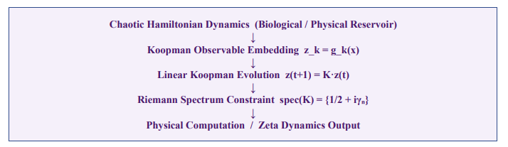
Figure 2: Conceptual architecture of the proposed bio-physical hybrid AI system. Biological chaotic dynamics (EEG, EMG, EKG) serve as the natural reservoir. Koopman observable projection enables linear readout, whose spectral properties are constrained to align with Riemann zeta zeros via an engineered Hamiltonian.

The Riemann Spectrum and The Hilbert -Polya Conjecture

Riemann Zeta Zeros and Spectral Theory

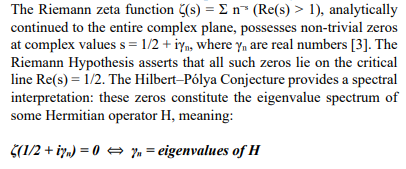
The statistical distribution of Riemann zeros has been shown to follow the level spacing statistics of the Gaussian Unitary Ensemble (GUE) of random matrix theory, which is characteristic of quantum chaotic Hamiltonians [9]. This establishes a deep connection between number theory, quantum chaos, and random matrix theory.

Yang–Mills Theory and Spectral Connections

Yang–Mills quantum field theory provides a natural candidate for the Hilbert–Pólya Hamiltonian. The Yang–Mills Hamiltonian H_ YM is self-adjoint and, in the confining phase, exhibits a discrete spectrum corresponding to glueball masses:

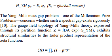
where the product runs over all primes p. The analogy between gauge field modes and prime number structure suggests that prime numbers function as fundamental modes of the zeta-dynamic system, with gauge field dynamics generating their encoding.

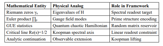
                      Table 2: Correspondence between Riemann zeta structures and physical systems.

The Grand Challenge: Hamiltonian Design and Spectral Readout

The central impediment to realizing the bio-physical hybrid AI framework described herein reduces to two inseparable requirements. We formalize these as the Grand Challenge of the proposed system:

Requirement I: Hamiltonian Generating a Riemann-Like Spectrum

The identification of an operator whose spectrum reproduces the Riemann zeros is an unsolved problem in mathematical physics, constituting the essence of the Hilbert–Pólya Conjecture. Several candidate models have been proposed. Berry and Keating's model employs the Hamiltonian H = xp, which classically generates chaotic flow and has been argued to reproduce the statistical structure of Riemann zeros in its semiclassical spectrum [11]. However, quantization of this operator in a standard Hilbert space yields a continuous spectrum, not the discrete zeros. Modifications involving boundary conditions and self-adjoint extensions have been explored, but no definitive realization has been demonstrated.

Alternative candidates include quantum Hamiltonians derived from lattice gauge theory and supersymmetric quantum mechanics. The lattice Yang–Mills Hamiltonian provides a discrete, self-adjoint operator with confinement-induced spectral gaps—structural properties compatible with Hilbert–Pólya requirements. Data-driven Koopman approximation offers a practical pathway: one trains a Koopman operator on physical system data and enforces spectral alignment with known Riemann zeros through constrained optimization.

Requirement II: Spectral Readout Methodology

Even given a Hamiltonian with Riemann-like eigenvalues,extracting these eigenvalues from a noisy physical system poses profound experimental challenges. The Riemann zeros are densely distributed along the critical line with statistical fluctuations matching GUE random matrix theory [9]. Distinguishing true Riemann zeros from eigenvalue fluctuations induced by experimental noise requires spectral resolution exceeding the local mean level spacing, which grows only logarithmically with height on the critical line.

Practical spectral readout strategies include: high-resolution power spectral density estimation via Welch's method or multitaper techniques, dynamic mode decomposition (DMD) for extraction of Koopman eigenvalues from time-series data, quantum phase estimation algorithms for quantum hardware implementations, and ensemble averaging analogous to EP signal averaging to suppress incoherent noise contributions.

In bioelectrical systems, the sampling constraint becomes a spectral constraint: the sampling frequency must exceed the spectral bandwidth of the Riemann spectrum being resolved. As the Koopman operator is the discretized form K = exp(Lt), where L is the generator of continuous dynamics, undersampling results in spectral folding—a higher-dimensional analog of aliasing—that corrupts Riemann zero identification.

PILLAR I Riemann-like Hamiltonian â??â??â??â??â??â??â??â??â??â??â??â??â??â??â??â??â?? Berry–Keating H = xp model Lattice Yang–Mills Hamiltonian Koopman constrained learning Supersymmetric QM candidates

PILLAR II Spectral Readout Methodology â??â??â??â??â??â??â??â??â??â??â??â??â??â??â??â??â?? Multitaper spectral estimation Dynamic mode decomposition Ensemble/coherent averaging Quantum phase estimation

Figure 3: The Grand Challenge illustrated schematically. Two solution pillars—Riemann-like Hamiltonian construction (Left) and spectral readout methodology (Right)—converge on the bio-physical hybrid AI system through the soil–iron union principle.

Soil and Iron: The Bio-Physical Hybrid Resolution

Conceptual Framework: Spontaneous Complexity and Structured Control

We propose that the Grand Challenge can be addressed through the systematic integration of two classes of physical substrates, which we term soil and iron in reference to their complementary roles. Soil denotes biological and naturally occurring chaotic systems that provide spontaneous high-dimensional nonlinear dynamics without requiring precision engineering. Iron denotes engineered physical devices that provide controllable, reproducible Hamiltonian structures with precision spectral properties.

Category	"Soil" (Biological Substrate)	"Iron" (Engineered System)
Physical Examples	Brain EEG field, bioelectric networks, cellular ion currents, plasma	Superconducting circuits, spin networks, Josephson junctions, microwave resonators
Key Property	Spontaneous chaos, massive parallelism, self-organization	Precision, controllability, reproducibility
Role in Framework	Natural Koopman reservoir, provides high-dimensional observables	Hamiltonian engineering, enforces Riemann spectral constraints
Grand Challenge Contribution	Addresses Requirement II (spectral readout via biological signal processing)	Addresses Requirement I (Riemann-like Hamiltonian construction)

Table 3: Complementary roles of biological (soil) and engineered (iron) substrates in the proposed hybrid framework.

Three-Layer Physical Architecture

The bio-physical hybrid AI system is organized into three coupled physical layers, each contributing distinct computational functionality:

1. Plasma/EM chaotic field layer: Provides continuous chaotic field dynamics serving as the high-dimensional reservoir. Biological electromagnetic fields (EEG, EMG, EKG) are natural instances, engineered plasma systems provide experimental controllability.

2. Spin network/Ising machine layer: Encodes combinatorial search spaces corresponding to NP-like computational problems. Spin configurations represent discrete state graphs amenable to optimization via physical energy minimization.

3. Superconducting circuit layer: Provides quantum-coherent Hamiltonian engineering via Josephson junctions, flux qubits, and microwave resonators. This layer enforces spectral constraints and enables precise eigenvalue measurement.

Together, these layers realize the structure: chaos + combinatorics + quantum coherence, enabling physical computation whose dynamics instantiate algorithmic processes.

Connection to Existing Computational Paradigms

Theproposedframework connects toand extends severalestablished computational paradigms. Neuromorphic computing exploits biological neural architectures for energy-efficient computation, but has not incorporated Riemann spectral constraints [12]. Physical reservoir computing has demonstrated computation using physical dynamical systems, including photonic, mechanical, and electronic reservoirs, but has not targeted zeta function dynamics [8]. Adiabatic quantum computing maps NP optimization problems to Hamiltonian ground state problems, sharing structural similarity with our Pillar I requirement [13]. Analog Ising machines solve NP problems through spin system energy minimization, corresponding to our combinatorial layer.

The bio-physical hybrid AI framework proposed here synthesizes these paradigms while adding the novel element of Riemann spectral alignment as the computational target—a unification we term Zeta Computing.

Polynomial Observables and Computational Complexity

The Koopman observable embedding requires selection of an observable basis. Polynomial observables g(x) = (x, x², x³, ..., xᵏ) are standard in EDMD and Koopman approximation theory. The dimensionality of the resulting observable space grows as C(d+k, k), where d is the state dimension and k is the polynomial degree [5]. For d = 20, k = 5, this yields thousands of dimensions—a combinatorial explosion structurally analogous to the complexity of NP search spaces.

This observation suggests a deeper connection: the polynomial observable expansion of a Hamiltonian dynamics system may naturally encode combinatorial search space structure, with the Riemann spectral constraint acting as a filter that identifies solutions. The formal statement of this connection—whether physical systems with Riemann-aligned Koopman spectra can efficiently solve NP problems—remains an open theoretical question whose resolution would carry implications for computational complexity theory.

The prime factorization structure encoded in the Euler product representation of ζ(s) provides suggestive evidence: if gauge field modes correspond to prime modes, then integer factorization problems—known to be computationally difficult—may be physically implemented through the zeta-dynamic system. This constitutes a speculative but theoretically grounded connection between the proposed framework and the P vs. NP problem.

Discussion

The framework presented in this paper synthesizes five distinct theoretical traditions—bioelectrical signal processing, Koopman operator theory, reservoir computing, Riemann zeta function spectral theory, and Yang–Mills quantum field theory—into a unified proposal for a new computing paradigm. Each tradition contributes essential elements: bioelectrical systems provide accessible natural reservoirs, Koopman theory provides the mathematical bridge between nonlinear dynamics and linear spectral analysis, reservoir computing provides engineering precedent for physical computation, Riemann spectral theory provides the computational target, and Yang–Mills theory provides the gauge-theoretic language for Hamiltonian construction.

The metaphor of soil and iron, while poetic, captures a genuine physical complementarity. Biological systems—evolved over billions of years to perform robust computation under noisy, energy-constrained conditions—exhibit precisely the spontaneous complexity required for a high-dimensional Koopman reservoir. Engineered physical systems—superconducting circuits, spin networks, electromagnetic resonators—provide the precision Hamiltonian control required to enforce Riemann spectral alignment. Neither alone is sufficient, their union addresses both pillars of the Grand Challenge.

Several limitations and open problems must be acknowledged. The Hilbert–Pólya Conjecture remains unproven, and no physical operator with a demonstrated Riemann zero spectrum has been identified. The connection between Yang–Mills spectral theory and Riemann zeros is conjectural, supported by statistical analogies but lacking formal proof. The proposed anti-aliasing and sampling constraints for bioelectrical Koopman reservoirs require experimental validation in prototype systems. The relationship between Riemann spectral alignment and computational complexity advantages requires rigorous theoretical analysis.

Future research directions include: experimental construction of small-scale bio-physical hybrid reservoirs using high-density EEG arrays coupled to superconducting spectral readout circuits, numerical EDMD studies of Koopman spectra for biologically realistic neural network models, lattice Yang–Mills simulations targeting Riemann zero statistical alignment, and theoretical analysis of complexity advantages for zeta-constrained Koopman systems.

Conclusions

We have presented a theoretical framework for bio-physical hybrid artificial intelligence grounded in the convergence of bioelectrical signal processing, Koopman operator theory, and Riemann zeta spectral computation. The central result is the identification of the Grand Challenge: the simultaneous requirement of a Riemann-like Hamiltonian and a viable spectral readout methodology. We have argued that this challenge is most naturally addressed through the union of biological chaotic substrates (soil) and engineered physical systems (iron), each providing complementary properties essential to the two pillars of the challenge. The framework connects to and extends neuromorphic computing, physical reservoir computing, adiabatic quantum computing, and analog Ising machine paradigms, unifying them under the novel concept of Zeta Computing. While significant theoretical and experimental challenges remain, the proposed framework provides a coherent research agenda whose realization would constitute a new paradigm in physical computation—one grounded in the deepest mathematical structures of number theory and quantum field theory.

References

- Niedermeyer, E., & da Silva, F. L. (Eds.). (2005). Electroencephalography: Basic principles, clinical applications, and related fields (5th ed.). Lippincott Williams & Wilkins.
- Wolpaw, J. R., Birbaumer, N., McFarland, D. J., Pfurtscheller, G., & Vaughan, T. M. (2002). Brain–computer interfaces for communication and control. Clinical Neurophysiology, 113(6), 767–791.
- Bombieri, E. (2000). Problems of the millennium: The Riemann hypothesis. Clay Mathematics Institute MillenniumProblems.
- Koopman, B. O. (1931). Hamiltonian systems and transformation in Hilbert space. Proceedings of the National Academy of Sciences, 17(5), 315–318.
- MeziÃÂ??, I. (2005). Spectral properties of dynamical systems, model reduction and decompositions. Nonlinear Dynamics, 41(1–3), 309–325.
- Webster, J. G. (Ed.). (2010). Medical instrumentation: Application and design (4th ed.). John Wiley & Sons.
- Luck, S. J. (2014). An introduction to the event-related potential technique (2nd ed.). MIT Press.
- Tanaka, G., Yamane, T., Héroux, J. B., Nakane, R., Kanazawa, N., Takeda, S., … Hirose, A. (2019). Recent advances in physical reservoir computing: A review. Neural Networks, 115, 100–123.
- Montgomery, H. L. (1973). The pair correlation of zeros of the zeta function. In Analytic number theory (pp. 181–193). American Mathematical Society.
- Jaffe, A., & Witten, E. (2000). Quantum Yang–Mills theory.Clay Mathematics Institute Millennium Problems.
- Berry, M. V., & Keating, J. P. (1999). The Riemann zeros and eigenvalue asymptotics. SIAM Review, 41(2), 236–266.
- Schuman, C. D., Potok, T. E., Patton, R. M., Birdwell, J. D., Dean, M. E., Rose, G. S., & Plank, J. S. (2017). A survey of neuromorphic computing and neural networks in hardware. arXiv.
- Farhi, E., Goldstone, J., Gutmann, S., & Sipser, M. (2000).Quantum computation by adiabatic evolution. arXiv.
- Lukoševicius, M., & Jaeger, H. (2009). Reservoir computing approaches to recurrent neural network training. Computer Science Review, 3(3), 127–149.
- Williams, M. O., Kevrekidis, I. G., & Rowley, C. W. (2015). A data-driven approximation of the Koopman operator: Extending dynamic mode decomposition. Journal of Nonlinear Science, 25(6), 1307–1346.