Reducing the Dimension of Infered Time-Varying Boundary conditions to Improve Water Levels Prediction in the Gironde Estuary using Telemac2D and an Ensemble Kalman Filter

Acknowledgements

We would like to thank the service in charge of flood forecasting in the Garonne, Adour and Dordogne watersheds (SPC GAD), and particularly Laurent DIEVAL for his help, as well as METEO- FRANCE and the Great Maritime Port Councils of Bordeaux (GPMB) for the bathymetric and observational data they provided for this study. The sea level observations along the Gironde estuary are the property of GPMB and the French Ministry in charge of sustainable development (MET). The authors sincerely thank Yoann AUDOUIN at EDF R&D and Matthias DE LOZZO at IRT Saint-Exup´ery for technical support.

Introduction

The Gironde estuary is the largest macrotidal estuary in France and Western Europe, with a surface area of 635 km2. Located in the southwest of France near the city of Bordeaux and the Blayais nuclear power plant, it is, on average, oriented from southeast to northwest. Its width varies from 1 km near Bordeaux to 15 km on the coast. Born from the confluence of the Dordogne and Garonne rivers, the estuary is under maritime influence and joins the Atlantic Ocean 75 km downstream [1]. The Gironde estuary is hypersynchronous and is influenced by an asymmetrical tide (4 h for the ebb and 8 h 25 min for the flow), dominated by the main semidiurnal lunar component (M2). The flow of the Garonne (resp. Dordogne) typically varies from 50 (resp. 20) to 2,000 (resp. 1,000) m3.s-1. In case of floodings, the flow of the Garonne may exceed 5,000 m3.s-1. The concomitance of high tidal coefficients and river floods can lead to significant flooding. The stakes in terms of environmental, economic and human safety are very high. Indeed, after the most severe flood ever recorded in 1770, infrastructures were constructed to limit overflows. Yet vulnerable areas could not be fully protected during the storms Lothar and Martin in 1999 or Xynthia in 2010 [2]. In order to implement preventive measures for warning and crisis management, government agencies rely on decision support tools. In France, the SCHAPI (Service Central d’Hydrom´eorologie et d’Appui `a la Pr´evision des Inondations) and the Flood Forecast Services (FFS) are responsible for monitoring and forecasting water levels and flows on 22,000 km of rivers. Twice a day, they produce a full-color hazard alert map, available online for government authorities and the general public (http://www.vigicrues.gouv.fr). To create these risk maps, they rely on numerical simulations and in situ measurements [3]. Indeed, hydrodynamic numerical software packages based on the Shallow-Water Equations (SWE) are commonly used tools for operational flood forecasting as well as to help in the management and protection of urban infrastructures located near rivers and coasts [4].

The FFS Gironde-Adour-Dordogne (GAD) is in charge of the Gironde estuary area surveillance. In order to meet with operational expectations, especially for extreme events, FFS GAD moved from a statistical model based on meteorological data to a physically based model that solves the Shallow Water Equations (SWE) based on the hydraulic software Telemac2D [5]. The Gironde estuary model was limited to the non-overflowing area, excluding the floodplains owing to computational constraints in an operational context. Despite this limitation, it resulted in improving water level forecast skill and increasing alert lead-times. While this model provides good results for past events in re-analysis mode, with errors of less than 10 cm for non-overflowing scenarios, simulating high tides (HT) periods is more challenging and in overflowing situations, errors of the order of 30 cm remain near Bordeaux. The ‘Gironde project’ recommended areas for improvement among which updating the model state and parameters with data assimilation (DA) algorithms [6]. This strategy is expected to be more efficient in terms of performance and computational cost than developing and running an overflowing numerical model in operational mode.

Already widely used by the meteorological community, DA methods are now common tools in the field of ocean, coastal and river hydrodynamics [7-9]. Extensive research has thus been carried out and reported in the literature to improve surface hydrodynamic models’ results, using ensemble, variational or hybrid methods, in order to characterize, in particular, the hazard with regard to the risk of flooding (including marine submersion) or to improve flood or water level forecasting.

The Ensemble Kalman Filter (EnKF) is the sequential filtering assimilation method used in this study [10]. Based on the assumption of a linear Gaussian statespace model, it propagates and updates an ensemble of vectors that approximates the control vector distribution through the stochastic estimation of the first two statistical moments, i.e., the mean and the covariance of the ensemble [8]. The implementation of the EnKF is highly compatible with HPC task farming. Moreover, the EnKF has been highly successful in many extremely high-dimensional, nonlinear, and non-Gaussian DA applications [11]. The EnKF relies on the choice of variables (model state vector, forcings, model parameters, for example) to be corrected. These variables are treated as random variables with associated probability density functions (PDF). These PDFs are sampled to build an ensemble of “perturbated” simulations for the forecast and analysis steps of the EnKF.

This paper presents an original framework for the assimilation of water levels observations in the context of flood prediction in the Gironde estuary, that aims at improving the predictive capability of water levels and discharges for the Gironde estuary, focusing on locations of interest where safety and economical assets are at stake [12]. The EnKF analysis aims at correcting fluvial and maritime boundary conditions (BC) as well as model parameters such as friction and wind influence coefficient, which is little addressed in literature. It should be noted that this implementation differs from the classical use of filters that account for errors in model states. Indeed, any correction to the state is bound to exit the hydraulic network within a short period that corresponds to the transfer time of the river network. It should also be noticed that the correction of errors in meteorological forcings or in bathymetry/ topography data is beyond the scope of this study.

This paper comes as a follow-up of that presented a GSA under the same assumption for the Gironde catchment and showed that friction coefficient and BC were the predominant sources of uncertainty [1]. Friction coefficients can’t be measured directly and must be estimated through their impact on the hydrodynamic state of the system. The same goes for the wind influence coefficient. Discharge time series that are prescribed as upstream BC suffer from uncertainty that results from water level measurement and from the water level to discharge (H-Q) transformation via a local rating curve established from a limited number of gauging especially at high flow. Uncertainty in the downstream maritime BC are due to measurement errors and to surge level estimation.

The main originality is that the uncertainty in the boundary conditions (BC) is assumed to be well approximated by a Gaussian Process characterized by an autocorrelation function and an associated correlation time scale. The dimension of the time-varying BC is reduced and the coefficients of the truncated KarhunenLo`eve (KL) decomposition of this process are then considered in the control vector, together with the friction coefficients and the wind influence coefficient of the EnKF to reduce uncertainty. This original method for reducing uncertainties at the time-dependent (maritime and fluvial) BC is justified, as estuarine processes are characterized by the propagation of tides and surge levels from offshore to the continental shelf and, thus, deeply influenced by the maritime BC (water levels, surge levels or velocities. The corrected BC and model parameters that come from the DA analysis are then used to run a direct model simulation in order to spatially modify the state of the system to reduce the propagated error over time [13]. In spite of what is usually reported in the literature, we have here decided not to include the model state in the control vector. Indeed, this would significantly increase the size of the control and thus require a larger ensemble. Also, the generation of perturbed model states within the ensemble requires additional work that was easily saved here as the state perturbation now results from the perturbation of model forcing and parameters. Finally, state only correction is well known to have a limited impact on medium to long term model improvement and that only model correction can leverage [14]. Most references in the literature on the coastal or estuarine area seek to improve the prediction of water levels through the direct correction of the hydraulic state of the system. It actually corresponds to the estimation of the initial (or “background”) condition. Following this strategy, describe the use of a deterministic EnKF that controls the hydrodynamical state by assimilating real altimetry observations to improve the prediction of oceanic surge levels on the Argentinean coast [15,16]. They demonstrated that with this strategy, the predictionskill of the state by correcting the initial condition appears to be limited. In perturbation on BC are used to build an ensemble of background state but neither BC nor friction coefficients are included in the control vector [15,16]. The same strategy was chosen in [17-19].

Friction coefficients are estimated with DA for 1D river hydrodynamics as well as in the case of a schematic estuarine field with a standalone with a dual state-parameter approach or with an augmented-state approach [20-26,14,7]. In these studies, friction coefficients are supposed to be constant over time and their “true” value represents a target to reach with DA. In our study, these coefficients are supposed to be time-varying in order to reflect the physical friction process of a macrotidal estuarian system.

The structure of the paper is as follows. Section 2 presents the hydrodynamical model of the Gironde estuary. It also describes the methodology to reduce the dimension of time-dependent Telemac2D forcings. The EnKF implementation is presented in Section 3. In Section 4, this methodology is applied to the Gironde Telemac2D numerical model. The experimental set-up is presented in Section 4.1 for an observing system simulation experiment (OSSE) and real experiment. The DA strategy is validated in the control and observation spaces in the context of OSSE in Section 4.2. The results for real experiment are shown in Section 4.3. Conclusions and perspectives are given in Section 5.

Hydrodynamical Modeling of the Gironde Estuary

Shallow Water Equations

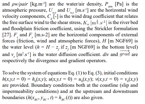
The Shallow Water Equations (SWE) are commonly used in environmental hydrodynamic modeling. The non-conservative form of the SWE is derived from two principles: mass conservation and momentum conservation, after expansion of the derivatives. The equations are written in terms of the water depth (h [m]) and the horizontal components of velocity (u and v [m.s-1]).

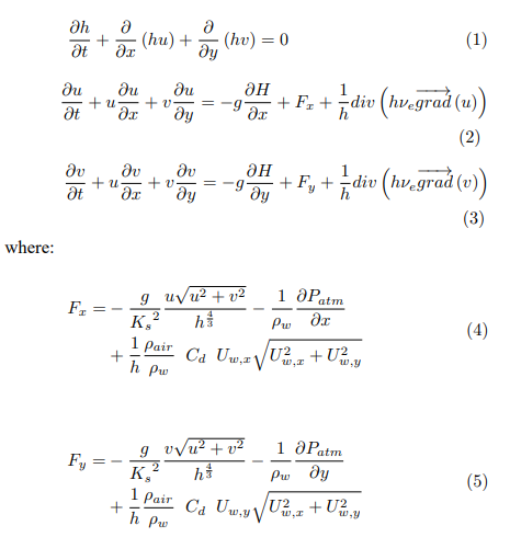
In the present study, as described in the SWE are solved with the parallel numerical solver TELEMAC2D (www.opentelemac.org) with a semi-implicit first-order time integration scheme, a finite element scheme and an iterative conjugate gradient method [1,5].

Numerical Modeling of the Gironde Estuary with Telemac2D

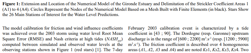
The numerical hydrodynamic model of the Gironde estuary is described and shown in Figure 1 [1]. It extends approximately 125 km from east to west, has 12838 finite elements and is composed of 7351 nodes. Based on the software Telemac2D, it is used by the FFS GAD for an operational purpose to compute the water height and velocity field from the mouth of the estuary to the upstream confluence of the Garonne and Dordogne rivers, respectively at La R´eole and Pessac. Hydrological upstream forcing for the Dordogne and Garonne rivers are provided by the DREAL (Direction R´egionale de l’Environnement, de l’Am´enagement des Territoires et du Logement) Nouvelle Aquitaine. It should be noticed that inflows from the Isle River and the Dronne River, both tributaries of the Dordogne river at Libourne, are artificially injected at Pessac and that flood plains are not taken into account [6]. The maritime boundary is located in the Gascogne Gulf, 35 km away from le Verdon. Surface forcing atmospheric fields (wind and pressure) from the regional meteorological model ARPEGE are provided by Meteo-France at a 6-hour time step. Water levels at the maritime boundary, which are the sum of the predicted astronomical tidal levels and meteorological surge levels, are also provided by Meteo-France at a 10 to 15 min time step.

Data Assimilation Framework

The methodology, called EnKF-γ-KLBC for stochastic Ensemble Kalman Filter (EnKF) correcting the control vector γ through the KL decomposition of the timedependent BC, consists in a sequential simulation algorithm, based on the well-known stochastic EnKF, for a joint estimation of parameters and time-dependent BC. It is original in that it resumes the correction of the time-dependent BC together with friction and wind influence coefficients to a simpler problem of parameters correction. Figure 2 summarizes the steps init init of the methodology which are detailed below.

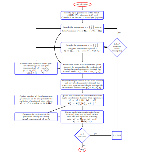
Figure 2: Dual Parameter and Boundary Condition Estimation Flowchart using the Stochastic EnKF with Reduced Boundary Conditionsin KL Space (EnKF-γ-KLBC) (adapted from) [14].

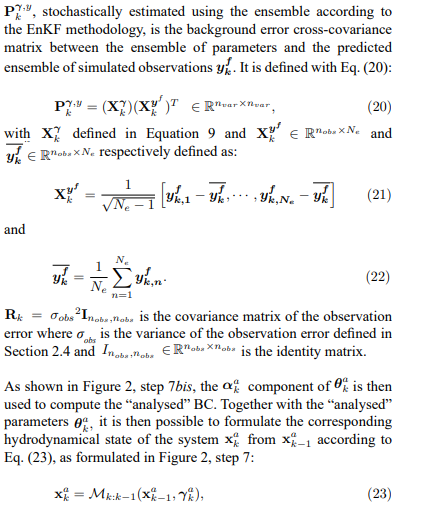
Description of the Control Vector γ

In this section, for the purpose of clarity, we consider that the index k refers to the time step t_k. Moreover, this index k has been removed from all equations at t_k

Controlled Variables

t_k, as shown in Figure 2, step 1. nvar is the dimension of γ and, therefore, the total number of controlled variables (parameters θ and modal coefficients α).

As described in Section 2.4, the correction of each time-dependent BC (QDOR, QGAR or CLMAR) is controlled by pBC parameters,also modal coefficients, applied to the pBC modes (Φi(t))_{i∈(1,,..pBC)} resulting from the KL decomposition of the autocorrelation function of the time-dependent forcing. On the one hand, α with dimension p_QGAR + p_QDOR + p_CLMAR gathers all modal coefficients for the BC included in γ and corrected with DA. On the other hand, θ contains the parameters of the numerical model assumed constant during a preliminary calibration phase (friction coefficients Ks and wind influence coefficient Cd of the hydrodynamic model, for example).

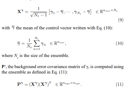
In the framework of ensemble-based DA, the anomaly X^γ of γ is defined with Eq. (9):

Initialization of the Control Vector

Based on the methodology for the creation of ensembles of parameters and perturbed time-dependent forcings and with uncertainties respectively described and Section 2.4, the initialization phase of the method consists in creating a background ensemble Xγ₀ at the initial time t₀ with dimension (n _var , N_e), as shown in Figure 2, step 2 [1]. The space filling strategy for the initialisation of θ₀ and α₀ is carried out with a Sobol’ sequence rather than a classical Monte-Carlo strategy, as showed it is more efficient in terms of dispersion and uniformity than the Latin Hypercube or Monte Carlo sampling methods although these are more popular in literature [35].

The control vector for each member i of the ensemble of size Ne at t₀ is denoted γ₀,i. The mean of the ensemble of the control vectors at t₀ is noted γ−₀ and its covariance matrix is noted Pγ₀ , respectively computed with Eq. (10) and Eq. (11).

EnKF-γ-KLBC Equations

The EnKF-γ-KLBC equations consist in a stochastic EnKF for the correction of the control vector γ. The two steps of the methodology are described below and in Figure 2. In the following notations, the a (resp. f) superscript stands for “analysis” (resp. “forecast”) step of the EnKF. It should be noticed that 0 0.

Forecast Step

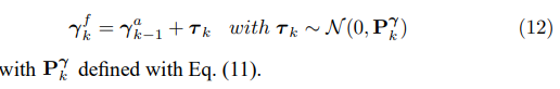
The KF usually applies on the model hydrodynamical state xk whose evolution is ruled by the shallow-water dynamical model during the forecast step, as described in Section 2.1. For model parameters such as γk, the propagation model doesn’t exist and is usually either replaced by a persistence model or a perturbation model [36].

In the first and general case, the use of a persistence model during the forecast step consists in propagating the control vector γ from t_k−1 to tk according to Eq. (12), as shown in Figure 2, step 3.

At each analysis, the EnKF reduces the variance of the ensemble As commonly known, this induces the collapse of the ensemble due to the lack of dispersion, all the more when the size of the ensemble is limited, and leads the EnKF to ignore the observations. for system state correction [8].

In this paper, a strategy to avoid the ensemble collapse is proposed. As shown in Figure 2, step 3, at each time step tk, γk is obtained by a resampling method based on the persistence of the initial 

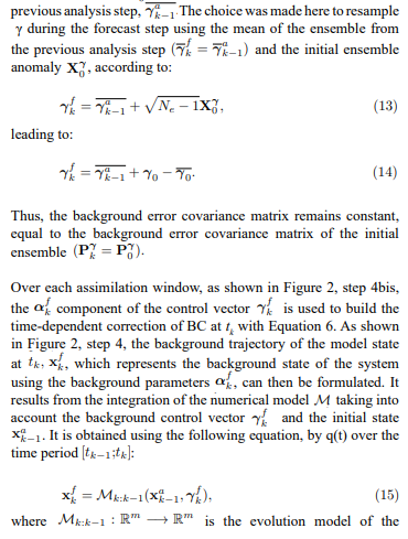
system hydrodynamical state from tk−1 to tk. m is the dimension of the system state vector.

Analysis Step

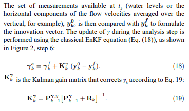
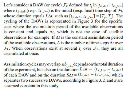
Data Assimilation Windows and Time Cycling

In this study, the equations described previously in Section 3.2 are used considering the k index relative to a DA Window (DAW) Fk over which all observations available are gathered in the observation vector y0. Indeed, the stochastic EnKF allows chaining Data Assimilation Windows {Fk }_{k∈{1,..,nb }} where nbcycles is the number of DA cycles of an experiment, as shown in Figure 3

Figure 3: Example of a Sequence of Two DAWs Fk−1 and _k for EnKF-γ-KLBC for L = 6 and S = 2 (Adapted from) [37]. If the Observations y⁰ are Available Every t = 1 h, then each DAW Lasts Lt = 6 h and the _k−1 DAW is Separated by S_t = 2 h from the _k DAW. The Observations Assimilated During Each DAW are Represented with Black Colored dots. In this Particular case, the (L − S) = 4 Last Observations Over the DAW Fk−1 are also Assimilated During _k. In the Special Case where L = S, the DAWs are Disjoint and Each Observation is Only Assimilated Once

The implementation of overlapping DAWs should be comprehended as the equivalent of the outer loop classically used with variational algorithm and reported in classical references [38- 41]. In a variational framework the outer loop aims at accounting for non linearity in the system by moving the reference with respect to which the non linear operators are linearized, to the analysis from the previous outer loop. In the present work, the relation between the control variables and the hydraulic state is non linear which triggers the optimality of the EnKF. The overlapping DAWs allow to gradually account for large misfits into the analysis, while preserving the optimality of the DA analysis in spite of non linear operators

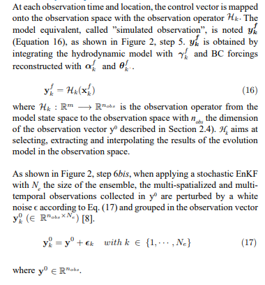
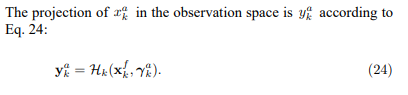
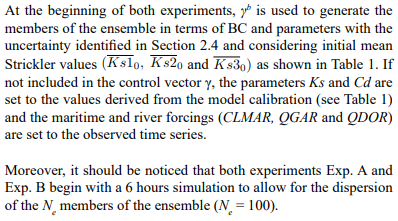
Application of EnKF-γ-KLBC to the Gironde Estuary

Two sets of experiments, Exp. A and Exp. B, were achieved respectively to validate and assess the performance of the EnKF- γ-KLBC methodology applied to the Gironde Estuary numerical model described in Section 2, in terms of water level prediction at different points of interest of the estuary located in Figure 1. For both synthetic (Exp. A) or real in situ (Exp. B) experiments, water levels observations are assimilated. The assimilation period is t = 1 hour. Experimental settings for Exp. A and Exp. B are summarized in Table 2 and detailed in Section 4.1.

             Table 2: DA Experimental Settings for OSSE 2003 Event During Exp. A and for 2016 Real Event During Exp. B.

Experimental Setting 

The controlled variables, grouped within the control vector γ, are corrected using the EnKF-γ-KLBC described in Section 3. For both Exp. A and Exp. B, the control run is the simulation without DA, with parameters and forcings set to the initial background control vector γb defined at γb . In Figures 4, 5, 7, 8 and 9 the b superscript is relative to the control run

Experimental Setting for the Synthetical Experiment (Exp. A)

Exp. A is an OSSE (Observing System Simulation Experiment) that assimilates synthetical water levels. Exp. A is based on the 7-day February 2003 calibration event. The duration of the validation OSSE equals 96 hours.

The control vector γ is composed of 7 uncertain variables: 3 friction coefficients (Ks1, Ks2 and Ks3), the wind influence coefficient Cd, and the time-dependent BC at the fluvial and maritime boundaries (QDOR, QGAR for the Dordogne, Garonne rivers respectively, and CLMAR). The time-dependent BCs are corrected through their modal coefficients applied to the main components of the autocorrelation function of the temporal signal, as explained in Section 3. Cycling parameters (Figure 3), L and S are set to 1 hour. Thus, there is no overlap between two successive DAWs so that, at each observation station, each hourly observation is assimilated only once.

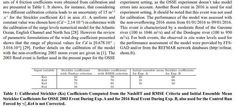
The initial background values γb₀ are gathered in Table 1 (friction) and Table 5 (BC and Cd).

Table 3: Location of the ”Assimilated” Observations for OSSE 2003 Event During Exp. A and for 2016 Real Event During Exp B. For Exp. A, Observations are Synthetic and Hourly Water Levels Extracted from the Simulation Exp. True. For Exp. B, Assimilated Observations are Hourly Real Observed Water Levels

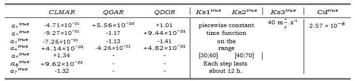
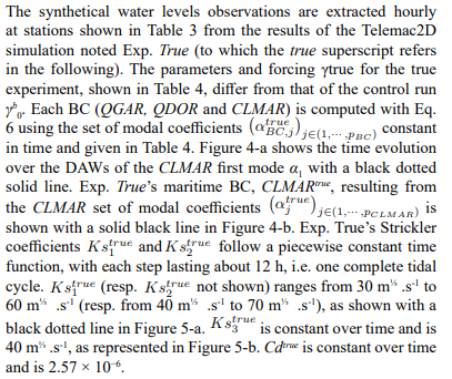
Table 4: “True” Parameters and “Modal” Coefficients Applied on CLMAR, QGAR and QDOR Modes Collected in γ^true for Exp. True for OSSE 2003 Event During Exp. A.

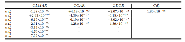
Table 5: “Modal” Coefficients Applied on CLMAR, QGAR and QDOR Modes and wind Influence Coefficient Cd at t₀, also used for the Control Run Forced by γ^b , for OSSE 2003 Event During Exp. A

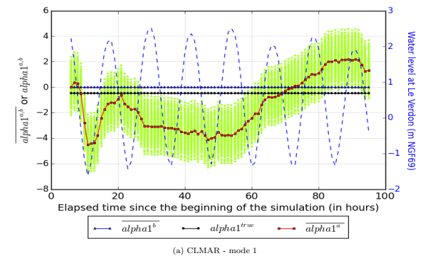
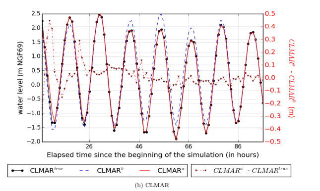
Figure 4: Time Evolution (Since the Beginning of the Event) of the CLMAR first mode α₁ (top) and of the reconstructed maritime boundary condition CLMAR^a (bottom) corrected using EnKF-γ-KLBC for OSSE 2003 event during Exp. A-1 over the DAWs (L=1h - S=1h). The maritime signal at Le Verdon is shown with a blue dashed line using the blue axis on the right. The green dots represent the ensemble of values taken by the control variable at each time step. CLMAR^true is the ”true” value of maritime boundary condition CLMAR for Exp. True from which the synthetic observations y⁰ are derived . CLMAR^b is the ”background” forcing of the control simulation.

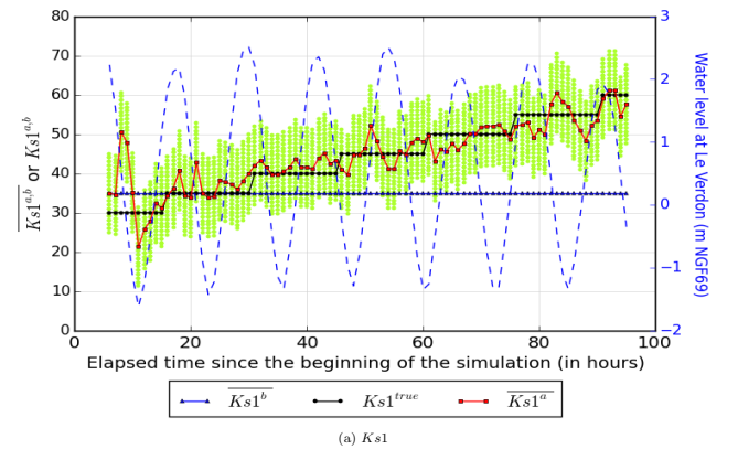
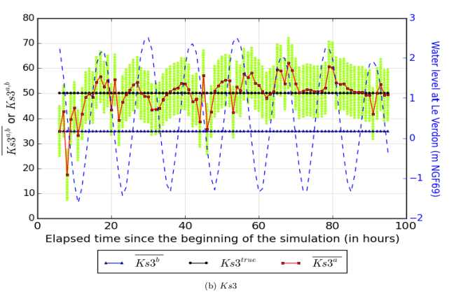
Figure 5: Evolution of Ks1 and Ks3 for OSSE 2003 event during Exp. A-1 during the assimilation cycles (L=1h S=1h). The maritime signal at Le Verdon is shown with a blue dashed line using the blue axis on the right. The green dots represent the ensemble of values taken by the control variable at each time step.

Exp. A has two main goals. On the one hand, it aims at confirming with DA the conclusions described concerning the influence area of each BC and parameter according to the tidal cycle [1]. That’s why, despite showed that the wind influence coefficient Cd or the river discharges (QGAR and QDOR) had no influence at all on the water levels in the estuary, they were included in Exp [1]. A’s control vector. In contrast, as Ks4 influences water levels at the upstream part of both Garonne and Dordogne rivers already respectively governed by QGAR and QDOR, it was not included in γ. On the second hand, Exp. A aims at optimizing the settings of the EnKF-γ-KLBC. For that reason, Exp. A was declined into several configurations, as shown in Table 3. Exp. A-1 uses all available observation stations, while Exp A−2, Exp A−3 and Exp A−4 present a limited number of observation stations. Indeed, Exp. A-1 uses 12 observation stations homogeneously distributed over the entire estuary, located at Le Verdon, Richard, Lam´ena, Pauillac, Fort M´edoc, Bec d’Amb`es, Le Marquis, Bassens, Bordeaux (limnigraph and tide gauge), La R´eole and Pessac.

Experimental Setting for real Experiment (Exp. B)

Exp. B assimilates “real” hourly observed water levels during the 2016 event described in Section 2.2 at the tide gauges located at Port-Bloc, Pauillac and Bordeaux PABx, as shown in Table 3 during the last 66 hours of the flood event where observations are available

Validation with an Observing System Simulation

Experiment (OSSE) environment (Exp. A)

Section 4.2 is dedicated to the discussion about the results for Exp. A. For figures representing the evolution of the controlled variables (Figures 4-a and 5), the mean background value of each controlled variable is displayed with a solid blue line, while the mean “true” value is displayed with a solid black line. The mean of the analysis is plotted with a red solid line. The green dots display the ensemble of values taken by the ensemble of analysis in the control space at each time step. The maritime signal at Le Verdon is displayed with a blue dashed line using the right blue axis. Figure 4-b displays the evolution of the maritime forcing CLMAR. The “analyzed” maritime boundary CLMAR^a is shown with a solid red line. The “true” (resp. background) signals CLMARtrue (resp. CLMAR^b) are displayed with a solid black (resp. blue) line. The difference between CLMARa and CLMAR^true is shown with a red dashed line using the right ordinate axis.

Sections 4.2.1 and 4.2.2 present the DA results for Exp A- in the control space (Section 4.2.1) and in the observation space 4.2.2 [1- 4]. The impact of the observation network characteristics is assessed in Section 4.2.3 and the influence of the DA hyperparameters is assessed in Section 4.2.4. Illustrations are shown for Exp A-1 only while results for all Exp A are expressed in terms of RMSE for water level at observations stations and are gathered in Table 6.

Station                          RMSE without DA                                 RMSE with DA

Table 6: RMSE with (Column “with DA”) and Without (Columns “Without DA”) EnKF-γ-KLBC for OSSE 2003 Event During Exp. A. The Last Line (“global”) is the Average of the RMSE Calculated on the 23 Stations of the Gironde Estuary. Stars (*) Besides RMSE Indicate the “Assimilated” Stations.

Results in the Control Space: Parameters and Forcings Estimation

The error between CLMAR^a and CLMAR^true is plotted with a triangle dashed red line. It is less than 10 cm at the end of Exp. A-1 for OSSE 2003 event. Similarly, QGAR and QDOR are reconstructed to within 2 % with respect to their true equivalent for OSSE 2003 event during Exp. A-1 (not shown here). These results show that, inspite of the equifinality in the space of the modal coefficients, the analysis allows to reconstruct a forcing that is very close to the true forcing for both maritime and fluvial BC.

Figure 5 displays the evolution of the friction coefficients Ks1 and Ks3 for “background”, “analysed” and “true” values over time for the OSSE 2003 event. Ks1a (Figure 5-a) is in good agreement with Ks1true despite the presence of noise of maximum amplitude of 10 m1/3 .s-1 . Similar results (not shown here) were obtained for Ks2a with a noise that reaches a maximum amplitude of 35 m1/3 .s-1 and seems to be decoupled from the tide signal.

The analysis for Ks3 is plotted in Figure 5-b and shows a noise of maximum amplitude 15 m1/3 .s-1 around the true value Ks3true = 50 m1/3 .s-1. This noise tends to weaken at the end of the OSSE 2003 event.

Results in the Observation Space: Water Level Prediction

As shown in Figure 2, step 7 and step 7bis, the analyzed parameters and forcings are used to simulate the analyzed water levels with Telemac2D. These are then compared to the synthetical observations for OSSE 2003 event during Exp. A. The maximum RMSE computed over the entire 2003 synthetical flood event between observed and predicted water levels with EnKF-γ-KLBC over the total duration of Exp. A-1, as shown in Figure 6, is less than 11 cm for all stations, except at B`egles and Cadillac where it reaches 12 and 13 cm respectively. Moreover, the EnKF-γ- KLBC reduces the time shift between predicted and observed HT (not shown here). Thus, despite a poor estimation of the modal coefficients associated with time-dependent forcings and some noise in the estimation of Ks3, as well as the equifinality mentioned in Section 4.2.1, the results in terms of water level prediction, obtained by correcting all the forcings and parameters of the Gironde estuary Telemac2D numerical model using its main stations, are very good.

Impact of the Observing Network

The various settings of experiments noted Exp. A aim at studying the influence of the location of the observing stations described in Table 3 on the performance of the EnKF-γ-KLBC along the Gironde estuary.

The RMSE between observed and predicted water levels with and without DA for each Exp. A are summarized in Table 6. The “assimilated” stations are noted with a star (*). The RMSE is computed for stations where the data is assimilated as well as where the data is used for validation only. Exp. A-2 presents the best water levels’ prediction performance for all stations, including the validation stations. In this configuration (L = S = 1 hour), the ideal observation network is that of Exp. A-2 that includes 7 tide gauges located in Royan, Richard, Pauillac, Bec d’Amb`es, Bordeaux (limnigraph), to which La R´eole (resp. Pessac) should be added, if the Garonne (resp. Dordogne) discharge needs to be corrected with EnKF-γ-KLBC. The analysis of the contributions brought by each assimilated station to the correction of each control variable Ks1, Ks2 and Ks3 (not shown here) shows, in agreement with the GSA results presented in that Ks1, Ks2 and Ks3 are mainly corrected using the water levels computed at the stations under maritime influence and that the contributions depend on the tidal cycle [1]. On the other hand, it was shown that the stations of Pessac and La R´eole don’t contribute at all to the correction of Ks1, Ks2 and Ks3.

Influence of DA Hyperparameters

It should be noted that a preliminary sanity check to study the influence of N_e (N_e ∈ [10,50,100,125,1000] members) showed that, beyond 50 members, Ne no longer influences the temporal evolution of the controlled variables nor the performance of the EnKF-γKLBC. It does not improve the equifinality issue that was previously highlighted. Ne = 100 members was further used to lower the computational cost and investigate the performance of EnKF-γ-KLBC for the water levels’ RMSE criterion in a synthetic framework Finally, the influence of the cycling of DAWs was considered for Exp. A-1. A 6-hours DAW shifted by 2 hours with the following DAW (L = 6 and S = 2 according to Figure 3) was considered. In this experiment, for each station, 6 observations are assimilated per cycle F_k and the last 4 observations are used for the next DAW F_k+1. The RMSE between observed and predicted water levels with DA is 1 cm lower for L = 6 and S = 2 than for L = 1 h and S = 1. The main benefit is that the high-frequency oscillations of −γ, described in Section 4.2.1 for Ks1^a and Ks3^a, are, by construction, smoothed (not shown here).

Results for a Real Experiment (Exp. B)

Results in the Control Space: Parameters and Forcings Estimation

For the real experiment Exp. B, as in Exp. A, the “analysed” modal coefficients αa governing the maritime BC CLMAR show some variability and do not converge to a constant value (not shown here). The resulting CLMARa and the instantaneous correction (CLMARa−CLMARb) are shown in Figure 7. The latter is a periodic signal, with a different period from tide, which proves that EnKF- γ-KLBC reduces the time shift between CLMARa and CLMARb. It supports the hypothesis of decoupling the uncertainties linked to the tide and the meteorological surge levels, as concluded in [1]. Moreover, CLMARa, compared to CLMARb, is not the result of bias or amplitude correction.

Figure 7: Maritime Boundary Condition CLMAR of the Numerical Model for 2016 Event During Exp. B.

The evolution of Ks1^a, Ks2^a and Ks3^a, controlled during Exp. B, are respectively displayed over time in Figure 8-a, -b and -c. On one hand, they show “high frequency” oscillations already highlighted in Section 4.2. This noise seems to be related to the use of the resampling method described in Section 3.2.1 and, also, to the cycling DAW with L = 3 h and S = 2 h. On the other hand, while Ks1a is generally in a range of “physical” admitted values for Strickler coefficients ([20 m^1/3 .s^-1; 80 m1/3 .s^-1]), Ks2a and Ks3a reach higher values. Ks2^a shows high values during the first part of Exp. B and values in the range ([60 m1/3 .s^-1; 80 m1/3 .s^-1]) after 100 h. Ks3a oscillates around 100 m^1/3 .s^-1. A too large value for Ks may reveal the decorrelation between friction in the river and the dynamics of the flow (water depth and velocity) in the estuary because of high water depths. Such values are not relevant in rivers where the water level is the result of a compromise between the upstream inflow, the downstream BC, bathymetry and friction. In these areas, a very large Strickler’s coefficient probably reveals an error in some other physical process not accounted for in the model. A threshold on Ks was applied here to constrain Ks2^a and Ks3^a to physical values. This highlights the sub-optimality of EnKF-γ-KLBC for this area subject to non-linear physical processes, especially at the confluence between the Garonne and Dordogne rivers. In this area, the correction of the friction coefficients tends to compensate other errors, such as the 3D flow turbulence or the diphasic stratification brought by the silt plug, especially in the Gironde estuary.

                                                                              (a)ks1

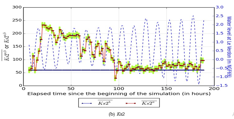
                                                                   (C.)Ks3

Figure 8: Evolution of Ks1, Ks2 and Ks3 for 2016 event during Exp. B during the assimilation cycles (L=3h S=2h). The maritime signal at Le Verdon is shown with a blue dashed line using the blue axis on the right. The ensemble is represented by green circles.

Results in the Observation Space: Water Levels Scores

The performance of EnKF-γ-KLBC is assessed over time using (y0 - ya) at the ”assimilated” observation station Bordeaux PABx and at validation stations Bordeaux2 and Cadillac in Figure 9. For complementary analysis, the water level RMSE is computed using the whole water level time series or using HT values only, at each station along the Gironde estuary. The RMSE for the 2016 event and Exp. B is displayed in Figure 10 and Figure 11.

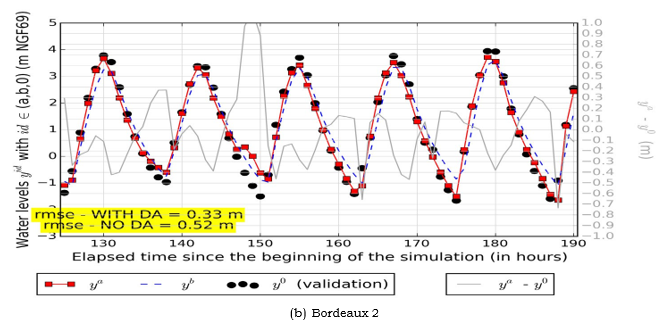
Figure 9: Evolution of Water Levels for 2016 Event During Exp. B (L=3h - S=2h) at a) the ”Assimilated” Station of Bordeaux, b) the Validation Station Bordeaux2, and c) the Validation Station Cadillac.

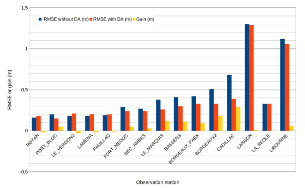
Figure 10: Root Mean Square error Along the Gironde Estuary for 2016 Event During Exp. B.

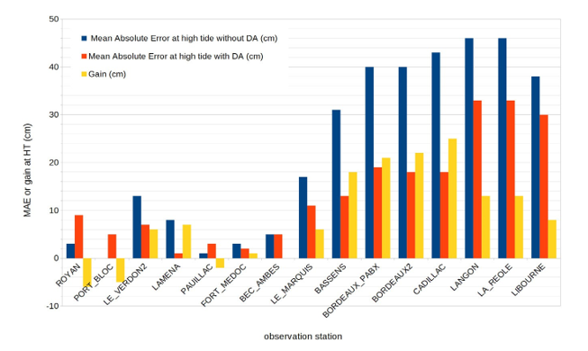
Figure 11: Mean Absolute error on HT Peaks Along the Gironde Estuary for 2016 Event During Exp. B.

Water levels at Bordeaux PABx, Bordeaux2 and Cadillac are represented in Figure 9-a, -b and -c. For the three stations, HT peaks are better represented when DA is used. Same goes for peaks at low tides (LT), particularly after 160 h. For Bordeaux PABx and Bordeaux2, the amplitude and shape of ya are also closer to y0 than yb. The Cadillac station is located between Bordeaux and La R´eole on the Garonne river. In spite of an unrefined mesh and no DA of observed water levels at la R´eole, at the upstream part of the Garonne river, the water level time series and the HT peaks, are better represented with EnKF-γ-KLBC. The water level RMSE at this station is thus halved, from 68 cm to 39 cm.

Figure 10 shows the water level RMSE obtained “without” (in blue) (resp. “with” in red) EnKF-γ-KLBC for all stations in the estuary where measurements were available during the event. The water level RMSE is computed from the instantaneous errors between ya (with DA) or yb (without DA) and y0 and significantly increases if the signal is time-shifted. EnKF-γ-KLBC allows for a small improvement in RMSE (less than 5 cm) downstream of Bec d’Amb`es. Yet, it allows for a significant improvement between the confluence and Bordeaux with a decrease in RMSE of 10 cm to 20 cm, and at Cadillac with a decrease in RMSE of 29 cm.

Figure 11 represents the mean absolute error (MAE) on water levels computed for HT peaks. While remaining lower than 10 cm, the MAE on HT peaks is degraded at Port-Bloc and Pauillac (eventhough observations are assimilated), as well as at Royan. Downstream of the confluence, the MAE decreases by 6 cm at Le Verdon and Lam´ena and is little influenced by EnKF-γ-KLBC at Fort-M´edoc and Bec d’Amb`es. On the Garonne river, the HT peaks estimation is substantially improved: the RMSE on HT peaks decreases from 30 cm to 46 cm between Le Marquis and Cadillac to RMSE on HT peaks lower than 18 cm. In conclusion, considering real observations in Exp. B, the methodology EnKF- γ-KLBC leads to a better representation of water level time series and HT peaks at almost all stations upstream of Le Verdon.

Conclusion and Prespectives

This article presents a DA strategy, denoted as EnKFγ-KLBC, for improving water level simulation by correcting scalar parameters such as friction and wind influence coefficients as well as time- dependent boundary conditions of a Telemac2D numerical model with a stochastic EnKF for the Gironde estuary. The dimension of the time series prescribed as upstream and downstream boundry conditions is reduced using the Karhunen-Lo`eve decomposition. The hydraulic state is not included in the control vector as any initial condition has limited impact on the simulated hydraulic state over time. Such extension could be investigated for very short term forecasts with high frequency of DAWs overlapping. The EnKF-γ-KLBC was successfully validated in OSSE mode for a non-overflowing 2003 event. It was shown that the time- dependent forcings are properly reconstructed and that the water level RMSE is significantly reduced and remains below 10 cm at almost all stations in the estuary. The commonly known equifinality issue was highlighted here in the space of the KL decomposition, especially when the control vector is extended with the friction coefficients. Nevertheless, the reconstructed forcing time series is satisfyingly close to that of the reference simulation. As a result, the analyzed water level is close to the synthetical observations. A series of OSSE experiments with different observation networks and assimilation settings are carried out and the most favorable choices are kept for the real mode experiment. The performance of the EnKFγ-KLBC was then assessed in real mode with the assimilation of in situ water level observations for the 2016 real non-overflowing event, in hindcast mode. The data assimilation analysis leads to a time-dependent variability of the Strickler coefficients and the coefficients of the KL decomposition for the maritime and fluvial boundary conditions. It was shown that the water level time series is better represented in terms of amplitude and that HT peaks are better estimated at almost all stations along the Gironde estuary. The merits of the proposed EnKF-γ-KLBC strategy were assessed for non-overflowing events. It appears as a reliable yet parsimonious alternative to setting up and running an overflowing 2D numerical model that classically implies access to high resolution topography data, resolution of complex physics and an associated high computational cost. For that reason, the proposed strategy paves the way for operational simulation of estuarine dynamics.

Sequential water level forecast is beyond the scope of this study and should be investigated with various strategies as presented in [42]. In that perspective, a free run (or an ensemble of free runs) would be issued starting from the last time of each assimilation window, for a chosen lead time period, for instance of +24h. While the correction of the hydraulic state is commonly known to be of limited use for mid- to long-term forecast, the correction of hydraulic parameters and forcing may allow for improvement. A straightforward strategy would consists in persisting the correction of the vector control beyond the end of the assimilation window, over the forecast period. In the present work, this resumes to applying the correction of the KL decomposition coefficients to build the boundary conditions over the forecast period. The corrected friction coefficients would be kept constant to the analyzed values over the forecast period. While this approach makes the most of the previously computed correction, it is questionable as the nature of the error in forcing and in friction may not be persistent over the assimilation and forecast periods.

Another perspective for this study stands in extending the control vector in order to take into account uncertainties in the surface forcing atmospheric fields (wind and pressure) over the Gironde estuary. A similar strategy to that applied for maritime and fluvial forcing could be applied, but this time over a 2D forcing field of atmospheric variables. In the context of ensemble forecast, the simulations for PE-ARPEGE issued at M´et´eoFrance could be used. As the size of the control vector increases, the cost of the ensemble based data assimilation strategy may become untrackable. The use of a surrogate model in place of the direct Telemac solver may be considered to limit the computational cost of the EnKF-γ-KLBC algorithm. This strategy was proven to be efficient in the context of sensitivity analysis with the 1D SWE software Mascaret or with Telemac over the Garonne river [43- 46].

Declarations

Conflicts of Interests

The authors have no conflicts of interest to declare that are relevant to the content of this article.

References

1. Laborie, V., Ricci, S., De Lozzo, M., Goutal, N., Audouin, Y., & Sergent, P. (2020). Quantifying forcing uncertainties in the hydrodynamics of the Gironde estuary. Computational Geosciences, 24(1), 181-202.
2. Hissel, F., Morel, G., Pescaroli, G., Graaff, H., Felts, D., & Pietrantoni, L. (2014). Early warning and mass evacuation in coastal cities. Coastal Engineering, 87, 193-204.
3. Golnaraghi, M. (Ed.). (2012). Institutional partnerships in multi-hazard early warning systems: a compilation of seven national good practices and guiding principles. Springer Science & Business Media.
4. Jain, S. K., Mani, P., Jain, S. K., Prakash, P., Singh, V. P., Tullos, D., ... & Dimri, A. P. (2018). A Brief review of flood forecasting techniques and their applications. International journal of river basin management, 16(3), 329-344.
5. Hervouet, J. M. (2007). Hydrodynamics of free surface flows: modelling with the finite element method. John Wiley & Sons.
6. Hissel, F. (2010). Projet gironde–rapport final d’évaluation dumodele gironde.
7. Evensen, G. (2009). The ensemble Kalman filter for combined state and parameter estimation. IEEE Control Systems Magazine, 29(3), 83-104.
8. Asch, M., Bocquet, M., & Nodet, M. (2016). Data assimilation: methods, algorithms, and applications. Society for Industrial and Applied Mathematics.
9. Liu, Y., Weerts, A. H., Clark, M., Hendricks Franssen, H. J., Kumar, S., Moradkhani, H., ... & Restrepo, P. (2012). Advancing data assimilation in operational hydrologic forecasting: progresses, challenges, and emerging opportunities. Hydrology and earth system sciences, 16(10), 3863-3887.
10. Evensen, G. (1994). Sequential data assimilation with a nonlinear quasi�geostrophic model using Monte Carlo methods to forecast error statistics. Journal of Geophysical Research: Oceans, 99(C5), 10143-10162.
11. Katzfuss, M., Stroud, J. R., & Wikle, C. K. (2016). Understanding the ensemble Kalman filter. The American Statistician, 70(4), 350-357.
12. Weerts, A. H., Winsemius, H. C., & Verkade, J. S. (2011). Estimation of predictive hydrological uncertainty using quantile regression: examples from the National Flood Forecasting System (England and Wales). Hydrology and Earth System Sciences, 15(1), 255-265.
13. Defforge, C. L., Carissimo, B., Bocquet, M., Bresson, R., & Armand, P. (2019). Improving CFD atmospheric simulations at local scale for wind resource assessment using the iterative ensemble Kalman smoother. Journal of Wind Engineering and Industrial Aerodynamics, 189, 243-257.
14. Moradkhani, H., Sorooshian, S., Gupta, H. V., & Houser, P.R. (2005). Dual state–parameter estimation of hydrological models using ensemble Kalman filter. Advances in water resources, 28(2), 135-147.
15. Zijl, F., Sumihar, J., & Verlaan, M. (2015). Application of data assimilation for improved operational water level forecasting on the northwest European shelf and North Sea. Ocean Dynamics, 65(12), 1699-1716.
16. Etala, P., Saraceno, M., & Echevarría, P. (2015). An investigation of ensemble-based assimilation of satellite altimetry and tide gauge data in storm surge prediction. Ocean Dynamics, 65(3), 435-447.
17. Bertino, L., Evensen, G., & Wackernagel, H. (2002). Combining geostatistics andKalman filtering for data assimilation in an estuarine system. Inverse problems, 18(1), 1.
18. Karri, R. R., Wang, X., & Gerritsen, H. (2014). Ensemble based prediction of water levels and residual currents in Singapore regional waters for operational forecasting. Environmental modelling & software, 54, 24-38.
19. Barthélémy, S., Ricci, S., Rochoux, M. C., Le Pape, E., & Thual, O. (2017). Ensemble-based data assimilation for operational flood forecasting–On the merits of state estimation for 1D hydrodynamic forecasting through the example of the “Adour Maritime” river. Journal of Hydrology, 552, 210-224.
20. Habert, J., Ricci, S., Le Pape, E., Thual, O., Piacentini, A., Goutal, N., ... & Rochoux, M. (2016). Reduction of the uncertainties in the water level-discharge relation of a 1D hydraulic model in the context of operational flood forecasting. Journal of Hydrology, 532, 52-64.
21. Cooper, E. S., Dance, S. L., Garcia-Pintado, J., Nichols, N. K., & Smith, P. J. (2018). Observation impact, domain length and parameter estimation in data assimilation for flood forecasting. Environmental Modelling & Software, 104, 199-214.
22. Ziliani, M. G., Ghostine, R., Ait-El-Fquih, B., McCabe, M. F., & Hoteit, I. (2019). Enhanced flood forecasting through ensemble data assimilation and joint state-parameter estimation. Journal of Hydrology, 577, 123924.
23. Siripatana, A., Mayo, T., Knio, O., Dawson, C., Le Maître, O., & Hoteit, I. (2018). Ensemble Kalman filter inference of spatially-varying Manning’sn coefficients in the coastal ocean. Journal of Hydrology, 562, 664-684.
24. Tamura, H., Bacopoulos, P., Wang, D., Hagen, S. C., & Kubatko, E. J. (2014). State estimation of tidal hydrodynamics using ensemble Kalman filter. Advances in water resources, 63, 45-56.
25. Jean-Baptiste, N., Malaterre, P. O., Dorée, C., & Sau, J. (2011). Data assimilation for real-time estimation of hydraulic states and unmeasured perturbations in a 1D hydrodynamic model. Mathematics and Computers in Simulation, 81(10), 2201-2214.
26. Hartnack, J., Madsen, H., & Sørensen, J. T. (2005, October).Data assimilation in a combined 1D-2D flood model. In Proc.Inter. Conf. Innovation, Advances and Implementation of Flood Forecasting Technology.
27. Gauckler, P. (1867). Etudes Théoriques et Pratiques sur l'Ecoulement et le Mouvement des Eaux. Gauthier-Villars.
28. Levy, F., & Joly, A. (2013). Modélisation des surcotes avectelemac2d. internal report, 24 pages.
29. Levy, F. (2013). Construction d’un modéle de surcotes sur lafaçade atlantique. rapport provisoire, avril 2013.
30. Efron, B., & Stein, C. (1981). The jackknife estimate ofvariance. The Annals of Statistics, 586-596.
31. Barthélémy, S. (2015). Assimilation de données ensembliste et couplage de modèles hydrauliques 1D-2D pour la prévision des crues en temps réel. Application au réseau hydraulique" Adour maritime" (Doctoral dissertation, Institut National Polytechnique de Toulouse-INPT).
32. Kucherenko, S., Feil, B., Shah, N., & Mauntz, W. (2011). The identification of model effective dimensions using global sensitivity analysis. Reliability Engineering & System Safety, 96(4), 440-449.
33. Sobol', I. M., Asotsky, D., Kreinin, A., & Kucherenko, S. (2011). Construction and comparison of high�dimensional Sobol'generators. Wilmott, 2011(56), 64-79.
34. Kucherenko, S., Albrecht, D., & Saltelli, A. (2015). Exploring multi-dimensional spaces: A comparison of Latin hypercube and quasi Monte Carlo sampling techniques. arXiv preprint arXiv:1505.02350.
35. Kucherenko, S., Albrecht, D., & Saltelli, A. (2015). Exploring multi-dimensional spaces: A comparison of Latin hypercube and quasi Monte Carlo sampling techniques. arXiv preprint arXiv:1505.02350.
36. Bocquet, M., & Sakov, P. (2013). Joint state and parameter estimation with an iterative ensemble Kalman smoother. Nonlinear Processes in Geophysics, 20(5), 803-818.
37. Bocquet, M., & Sakov, P. (2014). An iterative ensemble Kalman smoother. Quarterly Journal of the Royal Meteorological Society, 140(682), 1521-1535.
38. Rabier, F., Järvinen, H., Klinker, E., Mahfouf, J. F., & Simmons,A. (2000). The ECMWF operational implementation of fourâ? dimensional variational assimilation. I: Experimental results with simplified physics. Quarterly Journal of the RoyalMeteorological Society, 126(564), 1143-1170.
39. Mahfouf, J. F., & Rabier, F. (2000). The ECMWF operational implementation of four�dimensional variational assimilation. II: Experimental results with improved physics. Quarterly Journal of the Royal Meteorological Society, 126(564), 1171- 1190.
40. Rabier, F., & Liu, Z. (2003, September). Variational data assimilation: theory and overview. In Proc. ECMWF Seminar on Recent Developments in Data Assimilation for Atmosphere and Ocean, Reading, UK (pp. 29-43).
41. Trémolet, Y. (2008). Computation of observation sensitivity and observation impact in incremental variational data assimilation. Tellus A: Dynamic Meteorology and Oceanography, 60(5), 964-978.
42. Tiberi, A. L. (2021). Prévisions d'ensemble hydrologiques et hydrauliques pour la vigilance crues (Doctoral dissertation, Université Paris-Est).
43. El Moçayd, N. (2017). La décomposition en polynôme du chaos pour l'amélioration de l'assimilation de données ensembliste en hydraulique fluviale (Doctoral dissertation, Institut National Polytechnique de Toulouse-INPT).
44. Roy, P. T., El Moçayd, N., Ricci, S., Jouhaud, J. C., Goutal, N., De Lozzo, M., & Rochoux, M. C. (2018). Comparison of polynomial chaos and Gaussian process surrogates for uncertainty quantification and correlation estimation of spatially distributed open-channel steady flows. Stochastic environmental research and risk assessment, 32(6), 1723- 1741.
45. Goutal, N., Goeury, C., Ata, R., Ricci, S., Mocayd, N. E., Rochoux, M., ... & Malaterre, P. O. (2018). Uncertainty quantification for river flow simulation applied to a real test case: the Garonne valley. In Advances in Hydroinformatics: SimHydro 2017-Choosing The Right Model in Applied Hydraulics (pp. 169-187). Singapore: Springer Singapore.
46. El Garroussi, S., Ricci, S., De Lozzo, M., Goutal, N., & Lucor, D. (2022). Tackling random fields non-linearities with unsupervised clustering of polynomial chaos expansion in latent space: application to global sensitivity analysis of river flooding. Stochastic Environmental Research and Risk Assessment, 36(3), 693-718.