Quantum Energy of a Nanoparticle in Superposition Two States on R2

Introduction

We consider the quantum energy superposition of a linear combination of two states of the Hamiltonian, which is a solution of the Schrödinger equation. In addition, a mathematical linear differential equation is solved in time and position to find the energy of the eigenfunction of each state superposition. The quantum energy wave function Ψ(x,y,t) is the sum functional of two functions of the Fourier transform [3,4]. The superposition coefficients c1 and c2 are complex numbers that represent the probability amplitudes of each state [5,6]. Because of the confinement, the nanoparticle can always move in the box and must always have a minimum energy. We calculated the energy in the two-dimensional rectangular box α and β in nanometer thickness. Particle energy levels strongly depend on the size of the parameter lengths, which means that smaller wells lead to larger energy gaps between levels. The total quantum energy in the superposition of two states over R², which is mathematically represented by the average value of the Hamiltonian operator applied to the wave function. It describes the probability distribution of the nanoparticles in the two states. It considers the specific potential energy landscape in the 2D plane where the nanoparticle is confined. It essentially reflects the average energy that the particle would have if measured in this superposition state

Method

Overview of Superposition States

A nanoparticle in an infinite rectangular well refers to a very small particle, on nanoscale. It confines itself in a hypothetical potential energy box with infinitely high walls, creating a rectangular shape where the particle can move freely only within the defined boundaries. It illustrates key concepts of quantum mechanics such as the quantization of energy levels and the behavior of the wave function due to confinement [7].

The superposition state is quantum mechanical, where the particle can exist simultaneously in a combination of several states. In this case, the nanoparticle is in a mixture of two distinct positions in the 2D plane R². The construction of the superposition state is represented by two individual states as wave functions, for example Φ₁ and Φ₂ [8,9]. The superposition in the time-dependent wave function is a linear combination of these states:

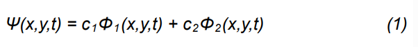
Here c₁ and c₂ are complex coefficients that represent the probability amplitude of each state.

The vertical red line in Figure. 1 represents the bounded state of infinite potential where the free nanoparticle moves in spin up and spin down between the rectangular box.

The complex nature of the coefficients c1 and c2 can lead to interference effects that help to understand the behavior of nanoparticle motions in quantum systems.

When the wave function is constructive Figure. 2, the amplitude of Ψ depends on the sum of the relative phase of the coefficients while it decreases in destructive interference Figure. 1. Case of destructive, waves can also cancel each other out in certain regions due to their phase relationships.

Computational Model

The boundary conditions of the rectangular well are given by 

Figure 1: Destructive Interference of Nanoparticle Around the Rectangular Well Box

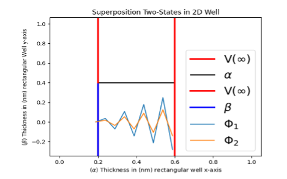
Figure 2: Constructive Interference of Nanoparticle Around the Rectangular Well Box

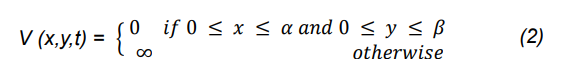
The free particle continues to move back and forth between the ends of the rectangular well. The total energy of the particle is less than the potential energy, which means that:

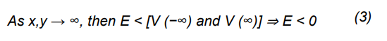
The quantum energy E(x,y,t) exceeds the energy potential V(x,y,t) on either side of the scattering state.

Next, we consider the density functional theory to compute the wave function of the quantum energy particle in the bulk configuration. We use the operator of the Schrödinger equation, the Hamiltonian, to find the wave function in a linear combination of two states.

 Waves

Theorem 1. If V(x,y,t) is an even function, then Ψ(x,y,t) can always be considered even or odd.

Proof. It is trivial by replacing (x,y) with (-x,-y). The wave function forms a linear combination of even and odd function.

The wave function Ψ can be solved using the method of separation of the variable of the linear combination of quantum energy (1). The solution is determined by the product of the sum of the waves and two functions of time t.

where Φ₁, Φ₂ are functions of x, y alone and f, g are functions of t alone. We let:

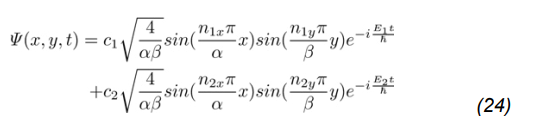
From equations (8),(9) and (10), the time- dependent wave function can be written in the form:

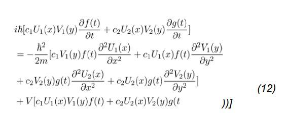
Using a time dependent Schrödinger equation of a Hamiltonian operation wave function (6), we substitute the wave Ψ(x,y,t) by its linear combination of partial wave functions (11) given [10,11,12]:

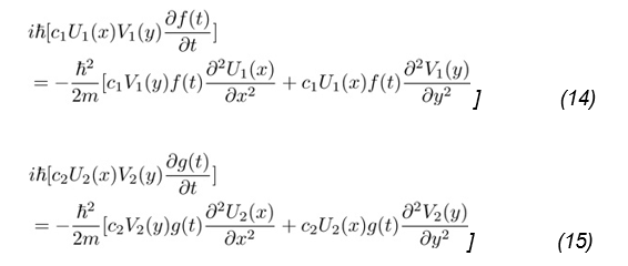
The boundary energy potential of the two states degenerates into the infinite rectangular well, that is:

Using the separation function method, we find two distinct quantum energy functions E1 and E2.

Theorem 2. The time-dependent wave function Ψ(x,y,t) is necessarily complex and can be expressed as a linear combination of different energy solutions.

Proof. We find it trivial using equations (14) and (15). We divide 

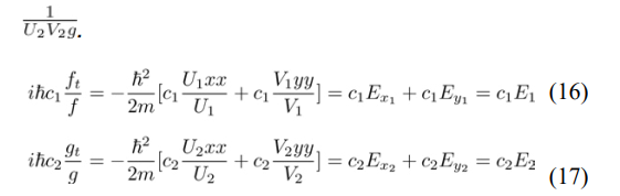
The time-dependent Schrödinger equation is found to be the partial differential equation and then solves the solution by using the ordinary differential equation [13,14].

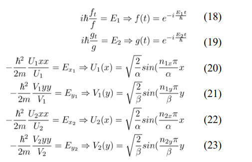
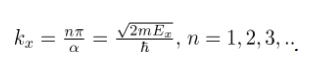
We apply the boundary conditions from the equations (20) to (23), for example U1(x) = A1sin(k1x) + A2cos(k1x) where x (0) = 0 and x(α) = 0 imply A₂ = 0 and

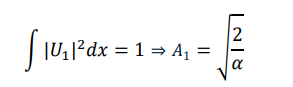
These conditions are similar to y-axis. We normalize the partial wave function given by:

We derive the quantum energy superposition from the particle wave function. According to the superposition principle, the linear superposition of several wave functions gives a new wave function that represents the possible physical state of the system [15,16].

Probability

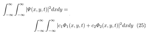
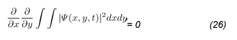
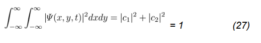
The probability density function of the particle’s location is the spatial integral of |Ψ(x,y,t)|2 in the rectangular box that gives the probability of finding the particle in the box at time t. Since the particle must be somewhere, the wave function for a bounded particle is usually normalized, so that:

It follows that the integral is constant and is independent of time.

Using the Kronecker delta function of two variables δNM, Φ₁Φ₁ = Φ₂Φ₂ = 1 and Φ₁Φ₂ = Φ₂Φ₁ = 0

Where |α|² is the probability of finding the nanoparticle in state one, and |β|² is the probability of finding the nanoparticle in state two [17].

Energy

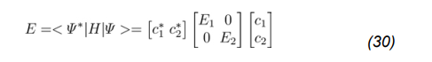
The quantum energy of the nanoparticle in the superposition is not a simple average of the energies of the individual states, but rather depends on the specific shape of the wave function and the potential involved. It can be calculated by solving the time- dependent Schrödinger equation (5). The expected value of the Hamiltonian determines the quantum energy

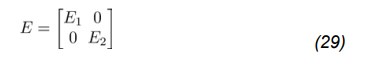
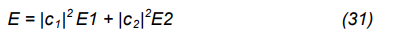
Where H is the Hamiltonian operator, and E1 and E2 are the energy of the basis states Φ1 and Φ2. For simple calculation, let us assume the Hamiltonian given by:

The quantum energy of the superposition state is given by

This is independent of time.

By simplifying the partial quantic energy, we finally obtain:

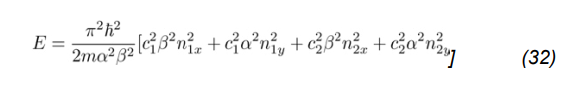
This explains why the quantum energy levels of the particle strongly depend on the size of the rectangular well, meaning that smaller wells result in larger energy gaps between the levels. The particle continues to move around in the box during confinement and still has some energy. Thus, lower energy levels correspond to smaller quantum numbers. The lowest energy level is called the ground state, and the highest energy levels are called excited states.

Results

We have used the application of the quantum energy of the particle in two-dimensional nanomaterials such as graphene shaped in a rectangular infinite well. We study the behavior of the nanoparticle wave function in graphene, which is a solid material that contains only a single layer of atoms arranged in an ordered pattern, where confinement plays a crucial role in their electronic properties. The nanoparticle wave function is restricted by the boundaries that prevent the scattering state, making its energy levels discrete and independent of size α and β. Due to its two-dimensional thickness, we opt for measurements of the lattices α = 0.2nm along the x-axis and β = 0.3nm along the y-axis. In the computation, we choose the coefficient amplitudes c1 = 0.02nm and c2 = 0.03nm.

Table 1: Energies States of the Wave Function

The table 1 shows the different levels of quantum energy. Level one is the lowest energy called the ground state (E=0.017657 eV). As node n moves up, the energies increase in the rectangular well, which are called excited states. Thus, the energy levels of the particle depend on the dimensions of the rectangular well and the quantum number n associated with each state.

Figure 3: Energy State: n_1x = 1 n_1y = 1 n_2x = 1 n_2y = 1 E = 0.017657 eV

This is the ground state of the particle’s wave function. The figure 3 shows us four different colors, and blue indicates that the energy of the particle is zero in the stationary state. Due to the confinement in the rectangular well, the particle can never be completely at rest and must always have a minimum energy in the box, where green and yellow join the darker red spot color occupied by the particle to reach the maximum energy of the lowest state.

Figure 4: Energy State: n_1x = 4 n_1y = 3 n_2x = 6 n_2y = 5 E = 0.473918 eV

This figure 4 represents the excited state of the quantum particle. Somehow, the wave graph of the central point can always have the highest energy. The amplitude of the wave is maximum. The probability of finding the particle in a particular region can be intensified by the highest energy (blue and red colors).

Discussion

The objective of this study is to evaluate the quantum energy of a nanoparticle that can exist simultaneously in several states. The superposition representation consists of the combination of the wave functions of the individual states, for example, Φ₁ and Φ₂ in the time-dependent Schrödinger equation. We consider the superposition of two states in a two-dimensional infinite rectangular well where the particle can move in antiphase or in the same direction, called destructive or constructive interference. We analyze the cubit state, which is a coherent superposition in two dimensions. The alpha value is the measure of the length between the two walls on the horizontal axis. The beta value is the measure of the length of the walls on the vertical axis with higher potential barriers. The quantum energy and the wave particle ratio are determined inside the box where the particle is trapped, and the potential energy is zero and infinite outside. The behavior of the nanoparticle is determined by the wave function Psi, which describes the probability amplitude of finding it at a given position. The wave is a linear combination of two states in which the Schrödinger equation, Hamiltonian, is solved in a two- dimensional Hilbert space. The superposition of two states can be illustrated by the example of a coin that can be heads and tails simultaneously until it is tossed and observed. The particle can move freely inside the box without any interference forces. In other words, the particle can be in a superposition of two different positions or have two different kinetic energies. The probability amplitudes c1 and c2 of each state are complex coefficients of the wave whose sum of individual squares is the normalization of the probability density function example of equation (27).

Quantum computing is used to evaluate the quantum energy of nanoparticles. The observed energy is the combination of the energies E₁ and E₂ of the basis states Φ₁ and Φ₂ (31). The quantum energy also depends on the alpha and beta lattices. The smaller they are, the higher the energy tends to be. By choosing a fixed value for α, β, and the amplitude of the coefficients, the quantum energy of the particle varies depending on the state level of the wave function. As the state level increases, the energy increases. The lowest energy is in the ground state, shown in Figure 3. The other state levels are called excited states, where the particle reaches its highest energy. In our example study, we have the two dimensional superposition structure of graphene: the particle exists simultaneously in two states rather than just one. Its unique electronic properties and massless Dirac fermions are used for potential applications in quantum computing and sensing. The particle can be in a combination of different energy levels within the electronic material of graphene. Graphene’s ability to exhibit a two states quantum superposition paves the way for the development of new quantum sensors and communication technologies for detecting various physical quantities. Graphene, a single layer of carbon atoms, allows the creation of a two-state superposition, such as graphene quantum dots (GQDs), leading to quantized energy levels. The quantum superposition of graphene enables the development of a new generation of quantum computations to perform previously impossible tasks.

Conclusion

In an infinite potential well of rectangular two-dimensional material, when a particle is in superposition of two quantum states, its quantum energy is a combination of the energies corresponding to those individual states. We calculated it by solving the time- dependent Schrödinger equation and taking a weighted average based on the superposition of coefficients α and β, with the energy levels themselves determined by the quantum numbers n1x, n1y, n2x and n2y associated with the x and y dimensions of the well. The quantum particle can exist in a combination of multiple quantum states simultaneously in the well. The most important aspect is that this model is often used to study the behavior of a particle in nanomaterials such as graphene, quantum dots, or sensors, where the confinement effects enhance their electronic properties.

In our next study, we will consider a quantum mechanical scenario in which a single particle is confined in superposition within a two-dimensional potential well with finite boundaries or tunneling effects through a potential barrier. Unlike an infinite potential well, the barriers have a potential energy, allowing a small probability of the particle being found outside the well boundaries [18-21].

References

1. Parr, R. G. (1989). Density functional theory of atoms and molecules. In Horizons of Quantum Chemistry: Proceedings of the Third International Congress of Quantum Chemistry Held at Kyoto, Japan, October 29-November 3, 1979 (pp. 5-15). Dordrecht: Springer Netherlands.
2. Hu, Y., Murthy, G., Rao, S., & Jain, J. K. (2021). Kohn-Sham density functional theory of Abelian anyons. Physical Review B, 103(3), 035124.
3. Muller, M. (2015). Fundamentals of music processing: Audio, analysis, algorithms, applications (Vol. 5, p. 62). Heidelberg: Springer.
4. Ullrich, C. A. (2011). Time-dependent density-functional theory: concepts and applications.
5. Messiah, Albert (1976). Quantum mechanics. 1 (2 ed.). Amsterdam: NorthHolland. ISBN 978-0-471-59766-7
6. Whitfield, J. D., Schuch, N., & Verstraete, F. (2014). The computational complexity of density functional theory. Many- Electron Approaches in Physics, Chemistry and Mathematics: A Multidisciplinary View, 245-260.
7. Shishodia, S., Chouchene, B., Gries, T., & Schneider, R. (2023). Selected I-III-VI2 semiconductors: Synthesis, properties and applications in photovoltaic cells. Nanomaterials, 13(21), 2889.
8. Ghosh, S., Verma, P., Cramer, C. J., Gagliardi, L., & Truhlar, D. G. (2018). Combining wave function methods with density functional theory for excited states. Chemical reviews, 118(15), 7249-7292.
9. Cina, J. A., & Harris, R. A. (1995). Superpositions of handedwave functions. Science, 267(5199), 832-833.
10. Marques, M. A., & Gross, E. K. (2003). Time-dependent density functional theory. In A Primer in Density Functional Theory (pp. 144-184). Berlin, Heidelberg: Springer Berlin Heidelberg.
11. Briggs, J. S., Boonchui, S., & Khemmani, S. (2007). The derivation of time-dependent Schrödinger equations. Journal of Physics A: Mathematical and Theoretical, 40(6), 1289.
12. Scrinzi, A. (2014). Time-Dependent Schrodinger Equation. Attosecond and XUV Physics: Ultrafast Dynamics and Spectroscopy, 257-292.
13. Zaitsev, V. F., & Polyanin, A. D. (2002). Handbook of exact solutions for ordinary differential equations. Chapman and Hall/CRC.
14. Polyanin, A. D. (2001). Handbook of linear partial differentialequations for engineers and scientists. Chapman and hall/crc.
15. Freegarde, T. (2012). Introduction to the Physics of Waves. Cambridge University Press.
16. Seck, P. M. (2021). Computational Mathematics in Density Functional Theory (Doctoral dissertation, Morgan State University).
17. Frankel, T. (2011). The geometry of physics: an introduction. Cambridge university press.
18. Hartmann, R. R. (2010). Optoelectronic Properties of Carbon-based Nanostructures: Steering electrons in graphene by electromagnetic fields. University of Exeter (United Kingdom).
19. Streltsov, A. I., Alon, O. E., & Cederbaum, L. S. (2009). Scattering of an attractive Bose-Einstein condensate from a barrier: Formation of quantum superposition states. Physical Review A—Atomic, Molecular, and Optical Physics, 80(4), 043616.
20. Tapia, O. (2009). Quantum linear superposition theory for chemical processes: A generalized electronic diabatic approach. Advances in Quantum Chemistry, 56, 31-93.
21. Neuhauser, D., Baer, M., Judson, R. S., & Kouri, D. J. (1991). The application of time-dependent wavepacket methods to reactive scattering. Computer physics communications, 63(1- 3), 460-481.