Orthogonal-Projection Localization for Polar Sensing Systems

The Problem

Polar sensing measurements record where transmitted energy interacts with a surface, but often omit the position from which that energy originated. Many data formats, such as PTS or ASC, list only the three-dimensional coordinates of the returns without including the sensor’s location or orientation. When such points exist in a shared coordinate frame, their spatial organization can still disclose the origin implied by the scan geometry. Each scanline or beam defines a radial path, and together these paths converge toward the point of emission. This same relationship governs optical, radar, and acoustic systems, which all measure reflections along straight or refracted radial directions. Even when the emitter itself is hidden, behind terrain, underwater features, or within clutter, its position can be inferred from backscatter observed by another platform. Each reflection provides a directional constraint toward the source, and the collective balance of these constraints reveals the origin already contained within the geometry of the observations. The same geometric relationship can also be seen in interference mapping and jammer localization, where bearings and signal gradients converge through the least-squares intersection to indicate the position implied by the spatial structure of the observations.

Prior Work

Estimating an unknown origin from directional data has appeared in several forms across imaging, radar, and acoustic research. The classical image-triangulation problem provides an early example. Hartley and Sturm (1997) examined the intersection of noisy image rays and derived least-squares solutions for point reconstruction from multiple views. Their analysis, later expanded by Hartley and Zisserman (2004), established the basis for geometric reconstruction by minimizing orthogonal distances between rays in three-dimensional space. Kanatani, Sugaya, and Niitsuma (2008) extended this work by introducing algebraic corrections and stability analysis, emphasizing robustness when the rays are nearly parallel or poorly conditioned. These studies reveal the same underlying mathematical structure present in the current formulation, though developed within the context of optical imaging geometry.

A separate line of research addresses emitter localization from range or timing information. Foy (1976) and Chan and Ho (1994) described both iterative and closed-form solutions for time-difference-of-arrival (TDOA) systems, in which hyperbolic range-difference constraints define the feasible region of the source. The relationship identified here differs in that it originates from directional rather than temporal data, yet the timing terms appear naturally as additional constraints within the same least-squares projection framework. In this sense, range-difference geometry represents another expression of the same spatial balance.

Bearings-only tracking studies also express this geometry. Nardone and Aidala (1981) analyzed observability and convergence properties for bearings-only localization, showing that geometry and relative motion determine when a unique solution can exist. Farina (1999) later summarized these and related approaches in a comprehensive treatment of passive tracking. The present method differs by using the projector form Pi = I − d_iid^T, which aggregates all bearing constraints into a single symmetric system Ap^ = b without requiring temporal sequencing or filter-based motion modeling. This makes it suitable for both static datasets and streaming updates.

Mathematically, the least-squares intersection relates to the “closest point to many lines” problem discussed in geometric optimization literature (Strang, 1986; Trefethen and Bau, 1997). However, the current treatment emphasizes the geometric balance revealed by the projection operators rather than the solver itself. Each term represents a component of the equilibrium already inherent in the data, and the intersection point represents the origin implied by the collective directions, independent of platform metadata or sensing type.

Recovering Sensor Origin from Structured Scanlines

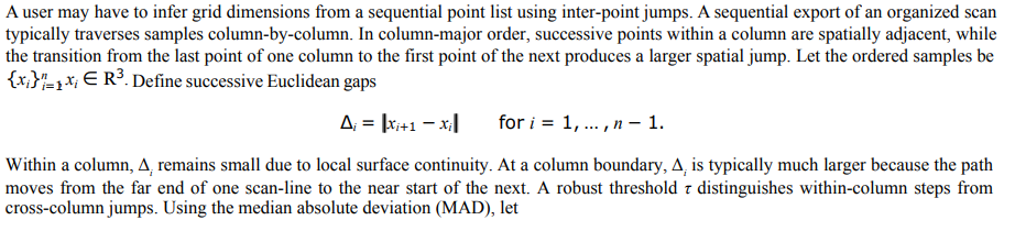
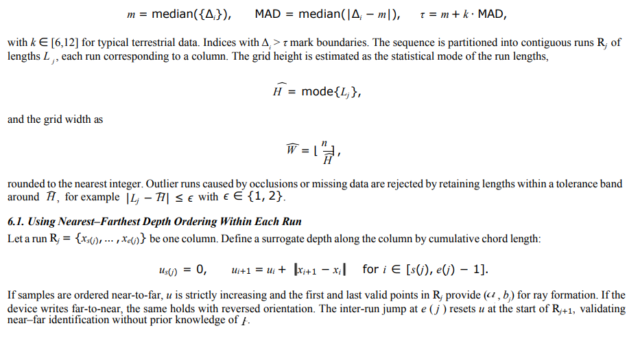
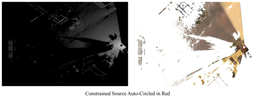
Polar datasets typically contain only sampled return positions without explicit metadata identifying the emitter or receiver origin. These datasets may already be globally aligned, yet without the origin position it is not possible to reconstruct the true propagation geometry. The method estimates the origin p from the point set itself by using the natural ray structure implied by each scanline. Each scanline defines a near–far pair of points that form a directional vector along which energy was transmitted or received. The least-squares intersection of all such lines yields an estimate of the sensor origin in the same coordinate frame as the data.

Importance of Sensor Origin

The sensor origin defines the direction of incidence for each recorded point, enabling computation of surface normals that face the sensor and determination of front, versus back-facing surfaces. The origin establishes energy propagation direction and is required to model beam divergence and footprint growth with range, which influence apparent roughness, intensity, and backscatter strength. Line-of-sight and shadow analysis depend on the origin for visibility tests and path-length modeling. Intensity normalization, backscatter modeling, and multi-return simulation require incidence angle and range referenced to the origin. In multi-scan or multi-sensor datasets, per-scan origin recovery enables angular incidence mapping, reflectivity corrections, exposure modeling, and verification of inter-scan alignment across radar, LiDAR, and sonar modalities.

Data Model

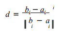
An organized point set is divided into vertical columns of width W and height H. For each column c, the first finite point ai and the last finite point bi define a line segment. The normalized direction vector is

Columns with invalid or degenerate pairs are excluded.

Finding Matrix Dimensions

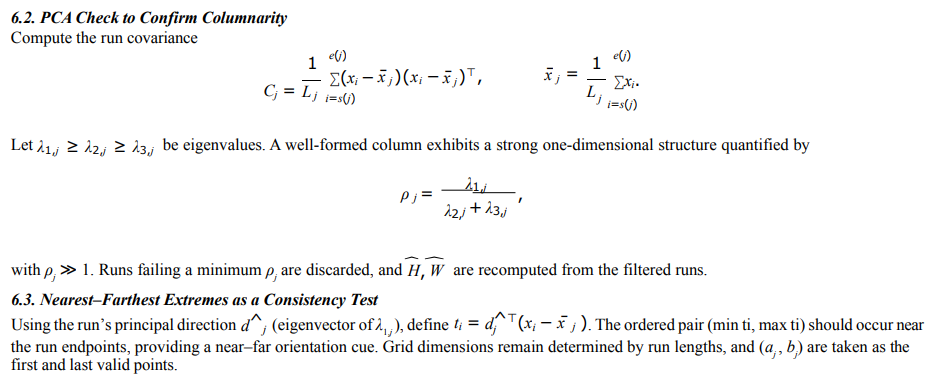
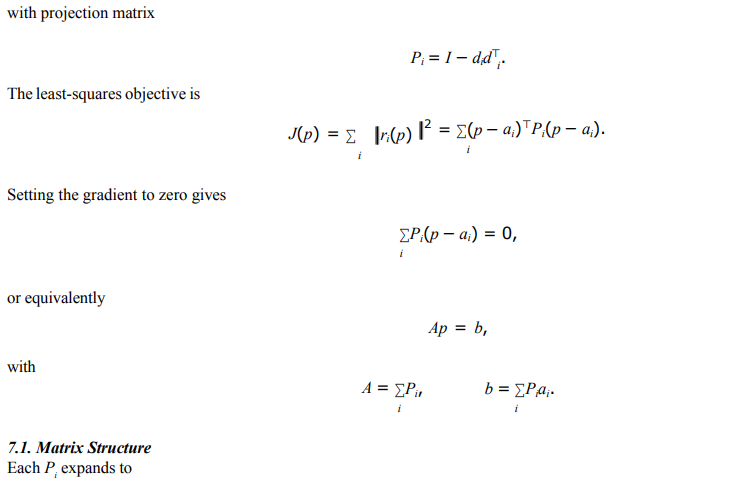
Scanner Location Using Geometric Basis

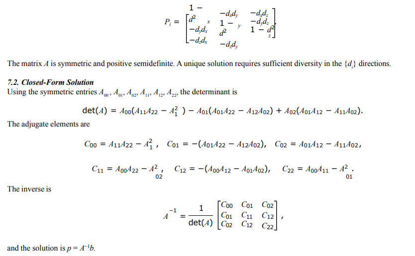
Application to Radar, Sonar, and Other Polar Modalities

The geometric principle extends to radar, sonar, and optical time-of-flight systems. For a steering direction di and one or more ranges ri,k along that direction, return points satisfy

                                               xi,k = p + ri,kdi.

When p is unknown but {xi,k} are embedded in a common frame, rays are formed using ai = xi, _min and bi = xi,_max and the same least-squares intersection is solved. The method applies to monostatic and bistatic configurations when the relevant ray directions are known or inferable.

Polar beams traverse layered media and reflect from intermediate and distant surfaces. Recovering p separates geometric propagation from environmental effects, enabling calculation of incidence angles, slant-range corrections, footprint size under beam divergence, multi-path discrimination via residual analysis, and energy loss modeling where attenuation and phase depend on path length and angle relative to the origin. When datasets are georeferenced or fused into a global frame, recovering p anchors local coordinate frames, supports Doppler–angle correlation, and calibrates directional response. The approach remains useful when metadata are absent or restricted while geometric relationships persist in the data.

Hidden Emitter Localization by Least-Squares Intersection

Hidden emitter localization relies on reconstructing the emission geometry of a LiDAR or electromagnetic source from indirect or secondary measurements. The least-squares intersection method estimates the origin p^ by minimizing the squared perpendicular distances between the hypothesized source and all observed propagation rays. The governing normal equations are

                                                       Ap^ = b,

where

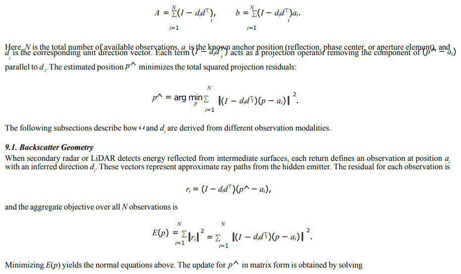
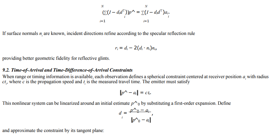
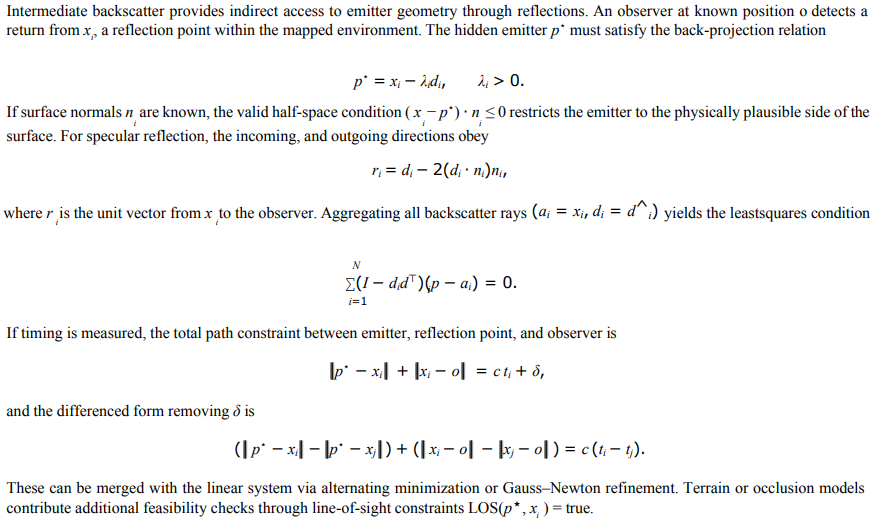
Hidden-Emitter Localization from Intermediate Backscatter

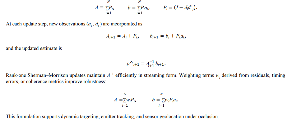
Post Hoc Recovery and Real-Time Operations

The same estimator serves both offline and streaming contexts. In post hoc recovery, previously acquired Cartesian point sets are re-processed to recover missing origin metadata, enabling accurate normal orientation, divergence modeling, and intensity correction. For real-time operation, accumulators are maintained incrementally:

Comments

The relationships derived above reveal a geometric balance that is present in all polar sensing data. Each observation of position and direction contributes to a spatial equilibrium that exists independent of the sensing system. This balance arises from how rays and obser-vation points are arranged in space. The least-squares intersection does not create this structure, it reveals it. The resulting point marks where all directional evidence is mutually consistent within the geometry already contained in the data.

This equilibrium represents a symmetry between emission and observation. The perpendicular offsets between a test origin and each propagation ray define a residual field that reaches its minimum where the geometry is most coherent. The least-squares process iden-tifies this position by reducing the total residual energy, tracing the system back to the geometric center implied by the data. The same relationship is observed across LiDAR, radar, and sonar data, all of which share a radial structure once expressed in terms of direction and position. The underlying symmetry appears whether the rays correspond to scanlines, reflections, or interference measurements.

In operation, this relationship can be updated continuously as new measurements arrive, maintaining an evolving estimate of the origin as evidence accumulates. Weighted versions of the intersection account for variation in confidence or coherence among observations, while timing and power-distance information refine the solution through additional constraints. Terrain and occlusion data define the boundaries of this balance, limiting possible origins to those that maintain clear geometric visibility to the observed points [1-9].

Emitter localization reveals the geometric equilibrium that exists within the data rather than creating a model to explain it. The summa¬tion form of the least-squares intersection provides a direct way to measure and describe this balance from observed directions and po¬sitions across different sensing systems and observation periods. The consistency that emerges reflects the geometry itself, independent of the platform or the method used to collect the measurements.

References

1. Foy, W. H. (2007). Position-location solutions by Taylor-series estimation. IEEE transactions on aerospace and electronic systems, (2), 187-194.
2. Kanatani, K., Sugaya, Y., & Niitsuma, H. (2008, September). Triangulation from Two Views Revisited: Hartley-Sturm vs. Optimal Correction. In BMVC (pp. 1-10).
3. Hartley, R. I., & Sturm, P. (1997). Triangulation. Computer vision and image understanding, 68(2), 146-157.
4. Hartley, R., & Zisserman, A. (2003). Multiple view geometry in computer vision. Cambridge university press.
5. Chan, Y. T., & Ho, K. C. (1994). A simple and efficient estimator for hyperbolic location. IEEE transactions on signal processing, 42(8), 1905-1915.
6. Nardone, S. C., & Aidala, V. J. (2007). Observability criteria for bearings-only target motion analysis. IEEE Transactions on Aero­space and Electronic systems, (2), 162-166.
7. Henry, S., & Christian, J. A. (2023). Absolute triangulation algorithms for space exploration. Journal of Guidance, Control, andDynamics, 46(1), 21-46.
8. Compagnoni, M., Pini, A., Canclini, A., Bestagini, P., Antonacci, F., Tubaro, S., & Sarti, A. (2017). A geometrical–statistical ap­proach to outlier removal for TDOA measurements. IEEE Transactions on Signal Processing, 65(15), 3960-3975.
9. Shi, H., Zhang, H., & Wang, X. (2016). A TDOA technique with super-resolution based on the volume cross-correlation function.IEEE Transactions on Signal Processing, 64(21), 5682-5695.