Model Reference Adaptive Inverse Control of Nonlinear Systems: A Deep Learning Approach

Introduction

Nonlinear control is concerned with system control applications in which the plant is nonlinear and hence does not obey the superposition principle. In order to make use of the powerful tools of linear system analysis, a first step is usually to linearize the system around an operating point [1-3]. Although useful, this method can only predict the nonlinear system behavior locally around that operating point. Moreover, in most cases, an accurate plant model or inverse plant model is required, in addition to the modeling of system parameters such as drag coefficients in controlling rigid bodies for unmanned aerial systems (UAS), for instance [4]. These are often difficult requirements, and therefore, the need arises for adaptive nonlinear controllers which usually take the form of neural networks (NNs), and can control nonlinear plants or slowly time-varying ones [5]. In addition, such adaptive controllers can counter the effect of system parameter uncertainties providing a robustness characteristic. This is a significant advantage especially when system uncertainties exceed the level of desired tolerance such that they would drastically affect the performance of a non-adaptive controller.

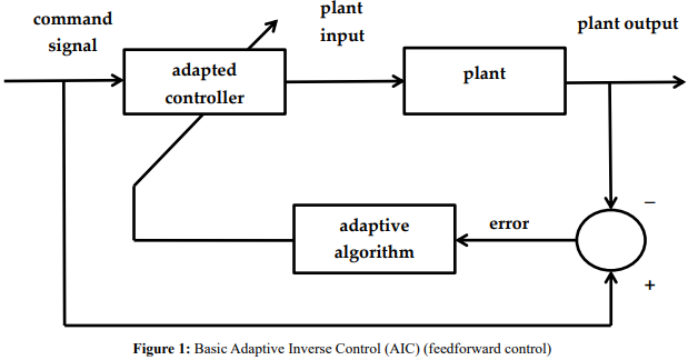
In particular, adaptive inverse control (AIC) is simple to implement when compared to the complexity of current control methods. This advantage becomes clearer when taking into account that, while nonlinear plants have no transfer function, approximate inverses are possible [6]. Inverse control is feedforward control as shown in Figure 1. The feedback is incorporated only in the adaptive algorithm to obtain the parameters of the feedforward controller. The control system of Figure 1 minimizes a function of the error between the command signal and the plant output. Upon convergence of the adaptive algorithm, the adaptive controller becomes the inverse of the plant provided the plant has a stable inverse.

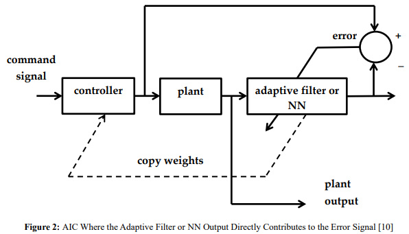
Adaptive algorithms such as the least mean square (LMS) algorithm for linear adaptive filters and the backpropagation algorithm for nonlinear systems or NNs work in a straightforward manner when the output of the adapted filter (or NN) representing the controller is directly related to the error signal [7-9]. Therefore, Figure 2 can be used instead.

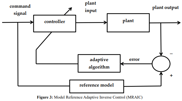
The control system of Figure 3 minimizes a function of the error between the reference model output and the plant output in an AIC setting. This is model reference adaptive inverse control (MRAIC). The order of the controller and plant, being nonlinear, cannot be changed as was done in Figure 2 since they generally would no longer be correct inverses of one another after adaptation. To retain the desired control-plant order of Figure 3, filtered-ε adaptation is applied, where the overall system error, designated by ε, is filtered before being used to adapt the adaptive nonlinear controller as will be explained fully in Section 3 [6]. This least squares adaptation method requires offline as well as online plant identification and inverse identification. NNs are used in the adaptive nonlinear controller, the nonlinear plant identifier and inverse identifier. This is readily justified since NNs are nonlinear function approximators that can model complex input-output nonlinear mappings.

Deep learning (DL) is proposed in this work by using deep NNs (DNNs), and comparing them with shallow NNs, to form an all-deep MRAIC system for the control of nonlinear plants. DNNs have been used in plant inverse identification in the context of DL AIC as in Figure 2 [10]. It has been proved that the deeper the DNN, the better the performance. In the present work, we prove that using a DNN controller adapted by the filtered-ε method also yields better performance compared to a shallow NN adaptive controller, while also using DNNs for plant identification and inverse identification.

Differently from our proposed easily-implemented deep MRAIC which is basically open-loop control, deep model reference adaptive control (MRAC) is dealt with utilizing the capacity of DNNs to model nonlinearities and resulting in powerful control of nonlinear plants with long-term learning properties, albeit involving negative feedback and closed-loop stability issues in [14,15]. To the best of the authors’ knowledge, deep MRAIC of nonlinear plants has not been dealt with in the literature. Many papers on MRAC control of linear and nonlinear systems have been reported, however. The design of MRAC control of an inverse-based non-minimum phase (NMP) system is presented, though with no resort to DL technique [16]. Since the plant is NMP and hence unstable, Lyapunov stability theory has been applied for the adaptation of the MRAC controller. Lyapunov-based MRAC control has also been used for aerial vehicles and D.C. motors in [12,17,18]. It has also been shown that the MRAC performance surpasses that of fuzzy logic and proportional-integral (PI) control, as MRAC plays an important role in determining the transient characteristics of the controlled plant output [19].

The paper is organized as follows. Section 2 presents a theoretical background of nonlinear discrete-time plant modeling, a brief explanation of deep neural networks and BP training and an overview of reference models. The filtered-ε adaptation algorithm and its incorporation in the proposed all-deep MRAIC control system of nonlinear plants are explained in Section 3. Section 4 presents and discusses implementation results. Finally, Section 5 concludes the paper.

Theoretical Background

A. Nonlinear Discrete-Time Plant Model

A dynamic discrete-time nonlinear plant is governed by a nonlinear difference equation. It is dynamic in the sense that its present output depends on n past outputs and m present and past inputs, where m ≤ n. This is in contrast to a static or memory-less system. Various models of such discrete-time nonlinear plants are given of which the following model was found to be particularly suitable for control problems [10,20].

where u(k) and c(k) denote the plant input and output respectively, k is the discrete time index, f [.] is a nonlinear function and βi are constants.

For satisfactory control of nonlinear plants, they have to be bounded-input-bounded-output (BIBO) stable. Moreover, they are assumed to be invertible and minimum-phase, that is, they have stable inverses. The term “minimum-phase” in linear system theory is used to mean that the system has all its zeros inside the unit circle. It can be used for nonlinear systems as to indicate that such systems have stable inverses, although a nonlinear system cannot always be assigned poles and zeros as in linear systems [5]. It is noteworthy that the plant model of Eq. (1) has a linear component.

B. Deep Neural Networks

The main idea in deep learning is that a function can be approximated by weighted combinations of an input feature vector using in-between nonlinear feature functions such as sigmoidal, tanh or the rectified linear unit (ReLU) functions [9]. Such a structure is a DNN that can be viewed as a nonlinear mapping with weights as parameters. For the control of dynamic nonlinear plants, DNN controllers, plant and inverse plant identifiers introduce dynamics via a tapped delay line whose input is the feature vector. A NN with more than one hidden layer is termed a DNN. It has been argued that a shallow NN with one hidden layer is a universal approximator [21]. However, a DNN has the merits of fewer parameters and nodes, and more layers also provide many features that are useful for approximation or regression as well as classification applications. The reason why a DNN has fewer parameters is that it learns composition of functions over the layers, which is simpler to learn than a single complex function. Hence generalization is achieved and overfitting is avoided due to the reduction in the number of parameters [9]. As a DNN will be denoted by 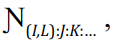where I, L, J and K represent the number of input nodes or neurons, the number of output nodes, the number of first hidden layer nodes, and the number of second hidden layer nodes respectively, and so on [10].

Regarding the DNN as a multiple-input-multiple-output (MIMO) system, the output vector of a three-layer (input plus hidden) DNN with two hidden layers can be written as [22]:

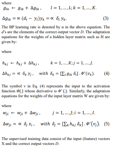
where X and Y are the input and output vectors respectively, G, H, and W are the weight matrices of the second hidden layer, the first hidden layer and the input layer respectively, and Φ and ψ are nonlinear activation functions to which the outputs of hidden and output layers are subjected. Only the output nodes are allowed to have a linear activation function depending on the application. The activation functions operate pointwise on the layer output vectors. The BP training algorithm is based on stochastic gradient descent [8,9]. It minimizes the squared magnitude of the error vector that represents the difference between the actual output vector Y and a correct output vector D, in accordance with supervised training mode. The BP adaptation equations for the weights of the output matrix G are as follows:

C. Reference Model

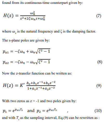
The reference model shapes the command input to the control system such that the plant output follows or tracks the desired shaped command input. The tracking control error, of which a function such as the mean square is to be minimized, is then the error between the reference model output and the plant output. As a shaping filter, the reference model has to be well designed to meet target performance specifications such as rise time and settling time, as well as to satisfy stability issues. Usually, it is taken as a linear time-invariant filter so as not to further complicate a nonlinear control system [12]. The model reference can take the form of a first- or second-order low-pass filter. For example, the z-transfer function of a first-order integrator that will be used in this work as a reference model is given by:

where K’ and a are positive constants.

The z-transfer function of a second-order reference model can be

Deep MRAIC Control of Nonlinear Plant

As mentioned in the introduction, to retain the normal controller-plant order in Figure 3, filtered-ε adaptation will be applied. It is helpful to first demonstrate this concept in the context of linear system control [6]. A linear MRAIC system is shown in Figure 4. An ideal non-existent hypothetical controller C(z) is shown dotted. Placing this controller instead of the block “copy ”, would minimize the overall system error ε. We assume that the difference between the outputs of C(z) and copy is the error ε’. Minimizing the mean square error of ε’ would make copy as close to C(z) as possible since they have a common input, but the problem is that this error ε’ is not available since C(z), which is the ideal controller, is not. However, it is easy to deduce from Figure 4 that filtering the overall system error ε by an inverse version of the plant P(z), denoted by , and using this filtered error to adapt would have the same effect. That is, the filtered error would be equivalent to the unavailable error ε’ for adaptation if the plant inverse were sufficiently accurate.

All adaptive filters considered in Figure 4 are linear FIR filters including a plant identifier and the inverse plant identifier obtained therefrom. These two adaptive identification settings are implemented offline first using a noise generator input and then online in connection with Figure 4. The connections, however, are not shown so as not to overcrowd the figure.

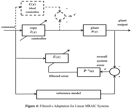
Figure 5 shows filtered-ε adaptation for a nonlinear MRAIC system where the plant is nonlinear. Adaptive NNs can be used for controller weights adaptation as well as the actual controller, and plant and inverse plant identifiers. As may be seen from the figure, the inapplicability of the superposition principle is accounted for by using separate blocks to filter the error components before combining them to form the overall filtered error.

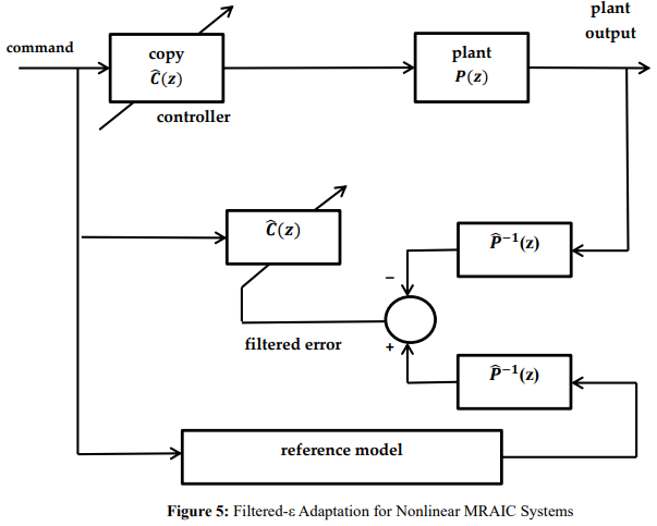
An all-deep control system is proposed where DNNs are used for controller weights adaptation as well as the actual controller, and plant and inverse plant identifiers in Figure 5. This would be the deep MRAIC system for the control of nonlinear plants. The benefits of using DL represented by DNNs in the proposed system will be clear when the results of its implementation are discussed in the following section.

Results and Discussion

The proposed nonlinear MRAIC system shown in Figure 5 is simulated and the results are presented. Simulations are performed in MATLAB (Version R2022a, Update 4, Academic license 30904939). The nonlinear plant to be controlled is chosen to obey the following nonlinear difference equation in conformity with the more general Eq. (1) with n = 2, m = 1 and βo =1:

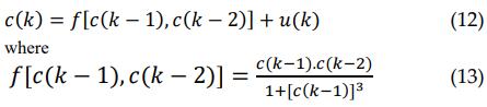
This plant will be designated as Plant 1.

The command signal is a discrete-time square function of 2000 samples, alternating between levels 0.5 and unity. The command is input to the controller and the reference model. The latter has a first-order transfer function given by Eq. (6) with K’=0.05 and a=0.95. The input buffer size or length of the input feature vector of all the DNNs in the control system is set to 3. So, the DNNs used can be described by the notation _{(3,1):5:5:5:5} with four hidden layers, ReLU activation functions and a single linear output node. The BP learning rate is 0.08.

Nonlinear plant and inverse plant identifiers using adaptive DNNs are first trained offline for a period of 10000 time samples using a noise generator input. These identifiers are then switched to the 2000-sample online mode where they are connected to the nonlinear plant of Figure 5. The inputs of plant and identifier are the same and the outputs of the two form the adaptation error. As for the inverse identification, it is implemented separately as a version of the identified plant whose output is input to the inverse identifier, and the adaptation error is the difference between the identified plant input and the inverse identifier output. The weights and structure of the DNN that implements the inverse identifier are copied on a sample-by-sample basis to the blocks of Figure 5 labeled .

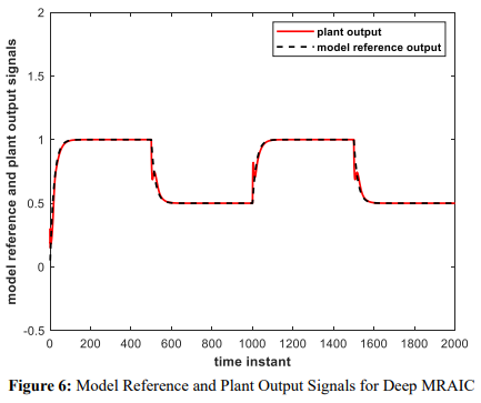
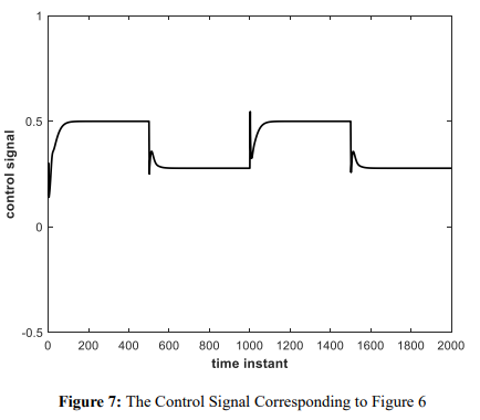
Figure 6 shows the model reference output plotted with the plant output in normal operation. The first-order exponential rise is of the reference model is clear. The plant output clearly tracks the model reference with the exception of the glitches appearing at the level transition instants of a square command signal alternating between 0.5 and unity. The control signal which is the controller output is shown in Figure 7.

We now aim at assessing the performance of the deep MRAIC system under plant parameter change. We assume that an abrupt parameter change occurs at the 1200th sampling instant such that Eq. (13) becomes:

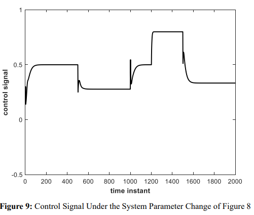
The model reference and plant output due to this parameter change are shown in Figure 8. The control signal is shown in Figure 9.

It is evident that since the plant output decreases momentarily due to the sudden parameter change, the control signal increases accordingly to resume tracking.

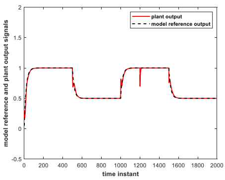
Figure 8: Model Reference and Plant Output Signals with Parameter Change at the 1200th Sample. (Deep MRAIC)

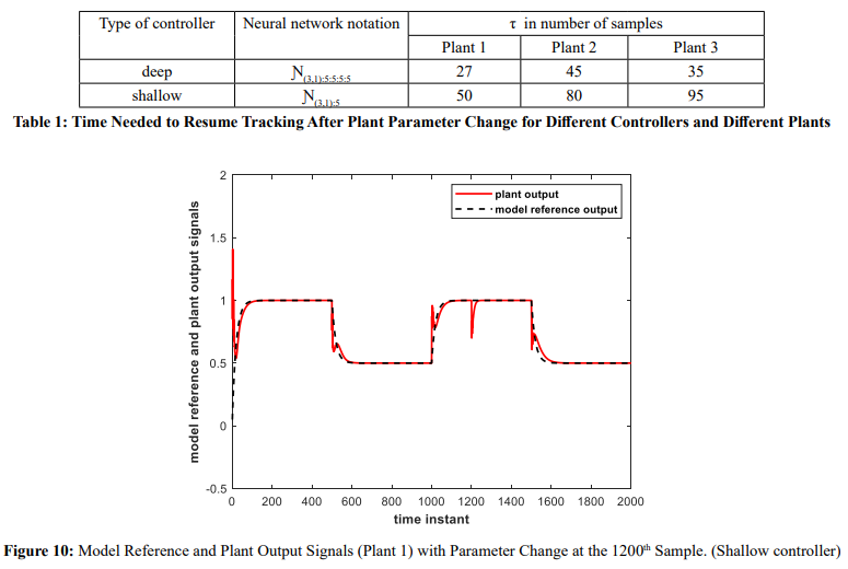
The parameter change is rapidly compensated for and the system resumes tracking. The time needed for the DNNs to re-converge and the system to resume tracking after parameter change will be called the resumed rise time and denoted by τ. Measured from results described by Figure 8, τ = 27 sampling intervals only, indicating robustness of the MRAIC system to abrupt plant parameter change.

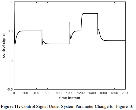
It is useful to compare the performance of the all-deep MRAIC system for the control of nonlinear plants to its counterpart with a shallow NN controller. To this end, we will replace the DNN controller with a shallow one denoted by _(3,1):5, and measure the resumed rise time τ. The result is shown in Figures 10 and 11 that demonstrate the tracking behavior and control signal respectively, under the same previously considered parameter change. The DNNs for plant and inverse plant identification are retained in both offline and online operation so that only the controller is made shallow. It is clear that the tracking performance shown in Figure 10 has deteriorated compared to Figure 8. The time τ has now increased to 50 sampling intervals. These results are further clarified in Table 1.

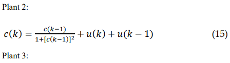
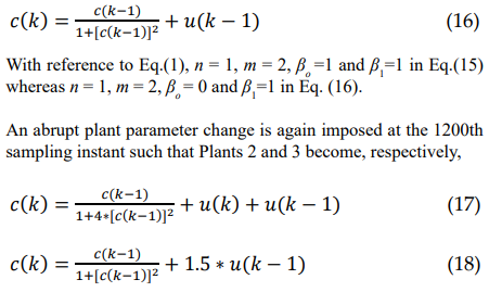
To prove the generalizability of these results, the MRAIC system is also tested with two other nonlinear plants designated as Plant 2 and Plant 3, with the following nonlinear difference equations:

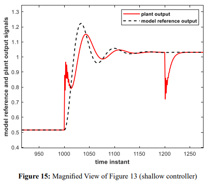
Next, a second-order reference model is simulated and experimented with using Eqs. (8), (10) and (11) with K’=0.0025, ω = 2 rad/s, ζ= 0.3 and T =0.05 s. Then, the tracking behavior of the overall all-deep MRAIC system and the system with a shallow controller are shown in Figures 12 and 13 respectively for Plant 1. The oscillatory transient due to the second-order reference model is evident. Abrupt parameter change is also included at the 1200th sampling interval.

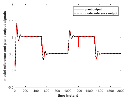
Figure 12: Second-Order Reference Model and Plant Output Signals. (all-deep MRAIC, using Plant 1)

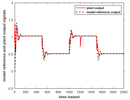
Figure 13: Second-Order Reference Model and Plant Output Signals. (Shallow controller, using Plant 1)

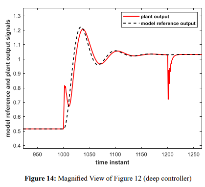
Magnified views of the second-order transient interval are shown in Figures 14 and 15. The superior tracking behavior of the all-deep system is evident.

Computational Complexity

The computational complexity of the MRAIC system can be discussed in terms of the number of multiplications per iteration executed by the deep controller as compared to that of its shallow counterpart. Addition operations are neglected, and the ReLU activation functions in the hidden nodes, as well as their derivatives, can be implemented by simple logic gates. The NN controllers perform multiplications in the feedforward mode of operation and in the backpropagation phase. The number of these multiplications per iteration can be estimated with the help of Table 2 in which we consider a hidden (or input) layer with J nodes, and assume that the hidden layer succeeding it has K nodes, followed by an L-node layer. Eq.(4) is representative of this situation in the weight updating phase.

Table 2: Number of Multiplications Per Iteration Associated with A General J-node Hidden (or input) Layer Followed by a K-node and Then An L-node Layer

An exception in the above table is the computation of δk if the K nodes are output nodes in which case no multiplications are needed when computing δk.

With the help of Table 2, it is found that the deep controller (_{(3,1):5:5:5:5)} of the MRAIC system requires 291 multiplications per iteration as compared to 51 multiplications per iteration needed by the shallow counterpart (_(3,1):5). The increased computational complexity of the deep controller is clearly offset by its improved performance compared to its shallow counterpart.

Conclusion

An all-deep MRAIC system for nonlinear plants has been proposed and simulated using first-order and second-order reference models. Comparison with the same system using a shallow controller demonstrated the improvement achieved by the deep controller in terms of the time needed to resume tracking after parameter change and tracking efficiency. Considerable improvement in tracking behavior of the all-deep version of the control system has been especially manifested when a second-order reference model was used. The proposed system combines the advantages of inverse control implementation simplicity and the superior adaptation and tracking ability brought about by deep learning techniques. The proposed system is also shown to be robust to abrupt plant parameter change.

References

1. Khalil, H. K. (2015). Nonlinear Control. Pearson Education Limited, London.
2. Rugh, W. J., & Shamma, J. S. (2000). Research on gain scheduling. Automatica, 36(10), 1401-1425.
3. Marquez, H. J. (2003). Nonlinear control systems: analysis and design (Vol. 1). Hoboken: Wiley-Interscience.
4. Lamb, Z. O., Bell, Z. I., Longmire, M. A., Paquet, J., Ganesh, P., & Sanfelice, R. (2025). Deep nonlinear adaptive control for unmanned aerial systems operating under dynamic uncertainties. In AIAA SCITECH 2025 Forum (p. 0106).
5. Plett, G. L. (2003). Adaptive inverse control of linear and nonlinear systems using dynamic neural networks. IEEE transactions on neural networks, 14(2), 360-376.
6. Widrow, B., and Walach, E. (2008). Adaptive Inverse Control, A Signal Processing Approach. IEEE Press.
7. Widrow, B. and Stearns, S. D. (1985). Adaptive Signal Processing. Prentice-Hall.
8. Kim, P. (2017). Matlab deep learning. With machine learning,neural networks and artificial intelligence, 130(21), 151.
9. Goodfellow, I., Bengio, Y., Courville, A. (2016). Deep Learning. MIT, Cambridge, MA, USA.
10. Alwan, N. A., & Hussain, Z. M. (2022). Deep learning for robust adaptive inverse control of nonlinear dynamic systems: Improved settling time with an autoencoder. Sensors, 22(16), 5935.
11. Mämmelä, A. (2006). Commutation in linear and nonlinear systems. Frequenz, 60(5-6), 92-94.
12. Nguyen, N. T. (2018). Model-reference adaptive control. In Model-reference adaptive control: a primer (pp. 83-123). Cham: Springer International Publishing.
13. Ioannou, P., & Fidan, B. (2006). Adaptive control tutorial. Society for Industrial and Applied Mathematics.
14. Joshi, G., & Chowdhary, G. (2019, December). Deep model reference adaptive control. In 2019 IEEE 58th Conference on Decision and Control (CDC) (pp. 4601-4608). IEEE.
15. Joshi, G., Virdi, J., & Chowdhary, G. (2020). Design and flight evaluation of deep model reference adaptive controller. In AIAA Scitech 2020 Forum (p. 1336).
16. Pal, M., Sarkar, G., Barai, R. K., & Roy, T. (2017). Design of different reference model based model reference adaptive controller for inversed model non-minimum phase system. Mathematical Modelling of Engineering Problems, 4(2), 75-79.
17. Orsag, M., Korpela, C., Bogdan, S., & Oh, P. (2013, May). Lyapunov based model reference adaptive control for aerial manipulation. In 2013 International Conference on Unmanned Aircraft Systems (ICUAS) (pp. 966-973). IEEE.
18. Luckson, N. L., Samba, G., & Falilou, N. M. (2023, February). Implementation of the robust MRAC adaptive control for a DC motor: A method based on the Lyapunov’s quadratic functional. In 2023 13th International Conference on Power, Energy and Electrical Engineering (CPEEE) (pp. 161-165). IEEE.
19. Keerthana, P. G. G., & Gnanasoundharam, J. (2016). Comparison of PI controller, model reference adaptive controller and fuzzy logic controller for coupled tank system. Indian Journal of Science and Technology, 9(12), 1-5.
20. Narendra, K. S., Parthasarathy, K. (1990). Identification and control of dynamical systems using neural networks. IEEE Transactions on Neural Networks, 1(1), 4-27.
21. Hornik, K., Stinchcombe, M., & White, H. (1989). Multilayer feedforward networks are universal approximators. Neural networks, 2(5), 359-366.
22. Alwan, N. A., & Hussain, Z. M. (2021). Deep learning control for digital feedback systems: Improved performance with robustness against parameter change. Electronics, 10(11), 1245.