Maxwell’s Quaternion Equations

Introduction

Electrodynamics is based on Maxwell's equations [1,2]. Maxwell generalized the experiments on electricity of Faraday and Ampere and described them in terms of vector mathematics in 1865. The discovery of the quaternion by William Rowan Hamilton occurred in 1843. In formulating the equations of electrodynamics, Maxwell used the Hamiltonian operator in 3D space with imaginary units i, j, k. This operator is a pure quaternion, i.e., a quaternion without a scalar part. The absence of the scalar part resulted in a zero solution to the equation based on Ampere's law. Therefore, Maxwell introduced into this equation the time derivative of the electric flux.

In everyday life, physical space is perceived as three-dimensional: length, width, height. In physics, time is added to the dimension of space. However, physical space is universal and allows for the formation of spaces of much greater dimensions within it. This fact is confirmed by the evolution of Nature on Earth and in outer space in general. The more complex the structure of matter, the greater the dimensionality of the space in which it is formed must be.

Mathematically, these phenomena can be described using hypercomplex numbers [3]. Quaternion forms a 4D space in 3D physical space, octonion – 8D, sedenion – 16D, etc. The dimension of the space is doubled by the dimension of the hypercomplex number. Doubling of dimensionality is associated with the procedure of doubling complex numbers when obtaining hypercomplex signals. Imaginary numbers i, j, k, etc. form orthogonal coordinate axes of such a space. The presence of scalar and imaginary parts in hypercomplex numbers allows us to explain how particles emerge from waves. Electromagnetic waves become material rather than a special kind of matter. The interaction of waves occurs not due to the ether, but directly due to the particles formed by them and vice versa.

The purpose of the article is to present a quaternion mathematical model of charges and their interaction with electric and magnetic fields, on the basis of which to obtain the equations of electrodynamics.

Materials and Methods for Solving the Problem

To derive the equations of electrodynamics, we use a quaternion. In algebraic form, a quaternion is written as [3,4]
q = s + ix + jy + kz ,    (1)
where s, x, y, z are real numbers, i, j, k are imaginary units.    
A quaternion function is also a quaternion, which can be written as a sum of functions p(s, x, y, z) , u(s, x, y, z), v(s, x, y, z) , w(s, x, y, z) :
f (q) = p + iu + jv + kw.    (2)
Quaternion (1) and function of quaternion (2) have dimension 4D in 4D space with real coordinate axis s and three imaginary axes i, j, k. To eliminate imaginary units in mathematical models of systems in multidimensional space, it is proposed to use their vector and matrix representation [5].

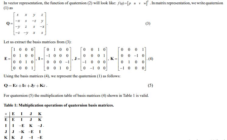
As can be seen from the basis matrices (4), representation (5) and Table 1, the imaginary units and, accordingly, the axes of spatial coordinates, also have a dimension of 4D. The basis matrices are orthogonal and do not intersect in space, i.e., when they are superimposed on each other.

Let us consider the use of quaternion (3) as a differential operator for the equation of dynamics in the state space [5]:
    x(t) = Ax(t)                      (6)

where A – state transition matrix (STM), and the variables x, y, z correspond to angular frequencies wi ,wj ,wk , the indices of which show the imaginary coordinate axes of 4D space, x(t) – time-varying quaternion in vector representation, x(t) – time derivative of a vector x(t).

Equation (6) is a matrix differential equation in time and state space. Multiplying the input vector by the STM produces an output vector in the form of a time derivative of the input vector. For constant values of angular frequencies wi ,wj ,wk , the STM has the simplest form:

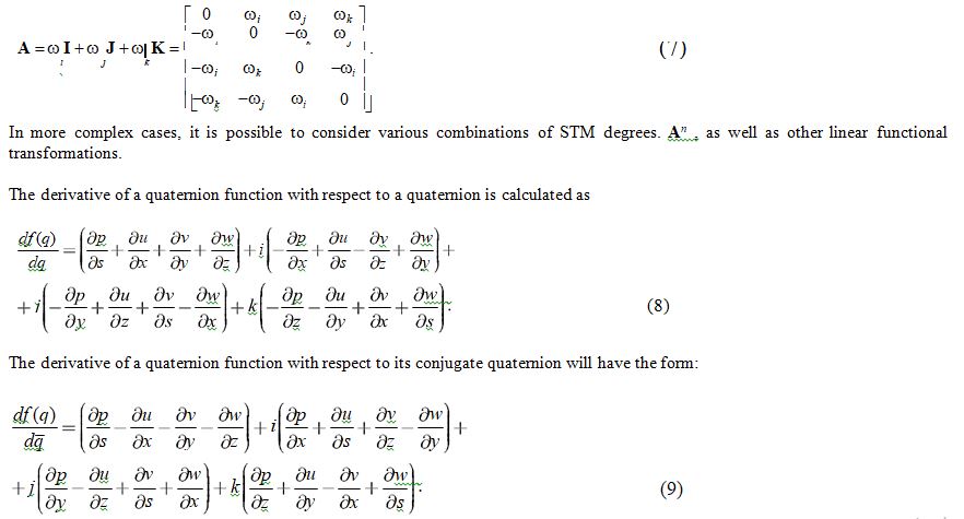
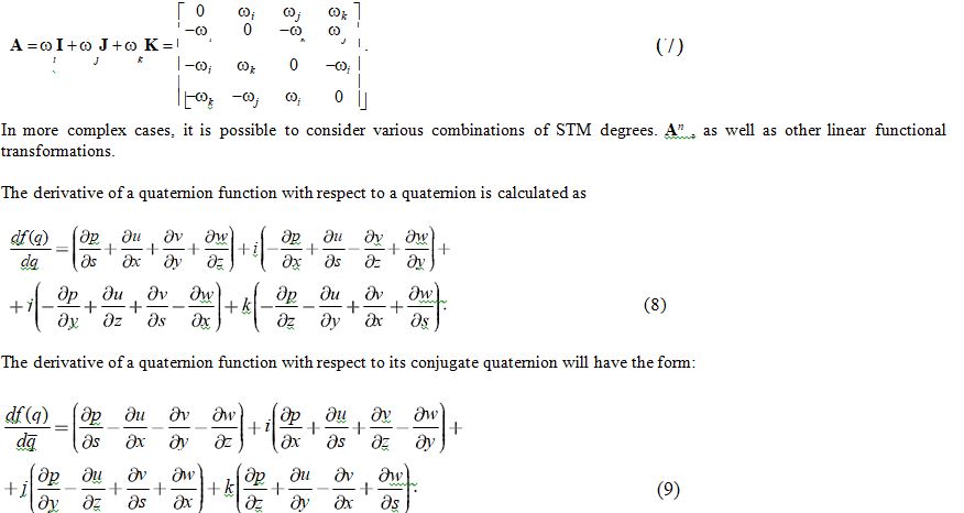
In matrix representation, we write the derivative (8) of function (2) using abbreviated notations of partial derivatives as

If function (2) is harmonic with component cosïÂÃÃÂ??ÂÃÂ?·t and sinïÂÃÃÂ??ÂÃÂ?·t , then when calculating the time derivatives of complex functions using (13), angular frequencies ïÂÃÃÂ??ÂÃÂ?·i , ïÂÃÃÂ??ÂÃÂ?·j , ïÂÃÃÂ??ÂÃÂ?·k appear in the form of multipliers of the STM elements (7) of the dynamic’s equation (6). Note that the angular frequencies are constant and the change in rotation angles occurs in accordance with the change in time.

The solution to the homogeneous linear matrix differential equation (6) will be the exponential of STM (7). The fundamental matrix of a three-frequency quaternion has the form [5]:

Thus, the quaternion space has a dimension of 4D. In this case, three coordinates are imaginary and one is real. For harmonic functions sine and cosine with different angular frequencies, each imaginary coordinate has its own angular frequency and a connection between time (rotation frequency) and space is formed. The STM for a dynamic state-space model is a differential operator and corresponds to the Hamiltonian operator. For harmonic functions, spatial differentiation corresponds to multiplying the elements of the quaternion by the angular frequencies of the corresponding spatial coordinate axes. The three-frequency fundamental matrix is a solution to the differential equation of dynamics in the state space. The three-frequency fundamental matrix for three reference frequencies is orthogonal and is decomposed into the sum (16) single-frequency orthogonal matrices (17) of combination frequencies (18).

Technique of Obtaining Maxwell’s Quaternion Equations
Quaternion Electrostatic Equations

In electrostatics, charge q is considered in 3D space and charges of various bodies are calculated using geometric transformations [1]. In this case, the three coordinates of 3D space represent the geometric coordinates of bodies. This representation does not take into account the dimensionality of the charge in the energy space and, accordingly, the connection between the coordinates of the charge with its energy coordinates and the spatial electromagnetic fields that form the charge.

Let us represent the charge q as a quaternion and consider it in 4D energy space as a vector q. Each axis of space will have a charge value and will be denoted by real numbers s, x, y, z, as in the algebraic representation of a quaternion (1). Since it is impossible to represent 4 axes on a plane, we will represent the scalar s as a sphere with coordinates for its imaginary axes. The radius of the sphere will determine the magnitude of the scalar [5]. To transform one 4D quaternion vector into another, a 4D matrix must be used. To satisfy the law of conservation of energy, in our case, charge, the matrix must be orthogonal.

Let us consider the imaginary unit of a single-frequency quaternion as the transformation matrix:

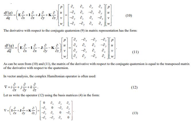
Figure 1 shows two charged particles of different sign and magnitude. Red indicates a positive charge, and blue indicates a negative charge. A positively charged particle is represented by a vector q1 = [ 5  -2  -3  2]T with the value of the scalar part of the charge s=5 and with the values of the imaginary charge coordinates in the matrix representation x=−2, y=−3, z=2. We use this vector as the initial state of the dynamic system (6). The ratio of the scalar part to the imaginary parts in the initial state can be anything. This ratio defines the norm of the charge vector. When multiplying by matrix (19), we obtain a charge Iˆq1 =[-1.7   0  -5.2 -3.5]T in which the ratio of the scalar part
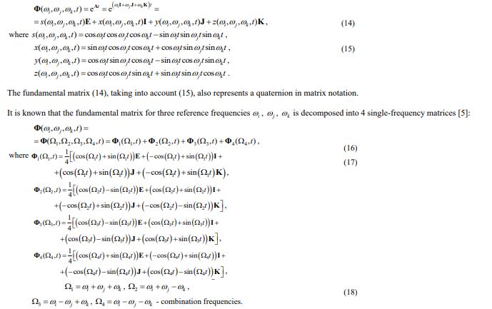
to the imaginary parts is determined by the constancy of the norm of the resulting vectors. As can be seen, the norm of the vector q1 is equal to the norm of the vector Iˆq1. Consequently, the charge q1 cannot move to any place in the charge space, but only to the one in which it maintains its norm. This transition can be called a quantum jump of a 4D electron. Similar transformations are shown in Figure 2 for the charge vector q2 = [-3 2 -1 3]T.

As is known, multiplication by an imaginary unit corresponds to a vector rotation. In our case, the rotation by matrix (19) can be divided into three rotations in 4D space, carried out by the basis matrices I, J, K.

Based on the dynamic’s equation (6), an electron can make many such jumps with different intervals depending on the change in time and the values of angular frequencies. Since the jumps occur without changing the energy, the movement occurs along an orbit with a constant radius, the length of which is determined by the energy (norm) of the initial vector.

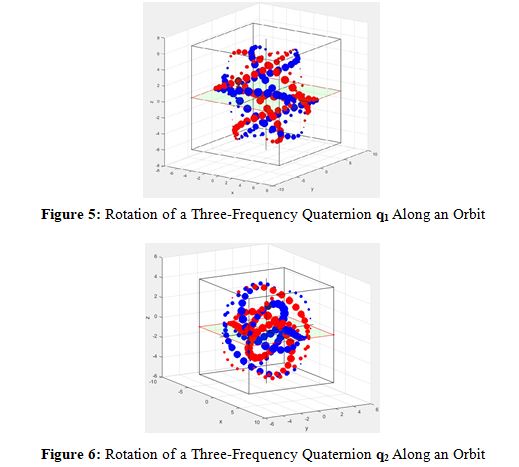
Figure 3 shows the orbit of a single-frequency quaternion for the initial state q1 = [ 5 -2 -3 2]^T corresponding to Figure 1. The initial state is depicted as a sphere with black surface lines. Figure 4 shows the orbit for the initial state q2 = [ -3 2 -1 3]^T shown in Figure 2.

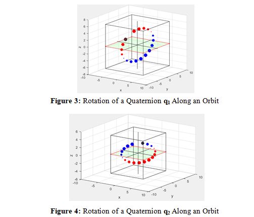
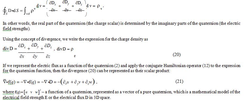
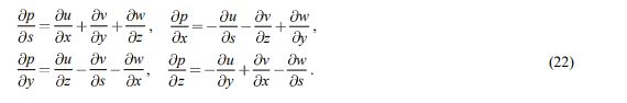
If rotation occurs without loss of energy, then it can last infinitely long. To move to another orbit with a different radius, it is necessary to obtain or spend energy. Note that the orbit is formed without using the fact of attraction of some bodies to others (gravity). When using a three-frequency quaternion (14), the rotation orbits will be more complex than with a single-frequency one. Figures 5 and 6 show examples of rotation orbits of the electrons discussed above [5].

It should be noted that the considered idea is consistent with M. Planck’s hypothesis about quantum radiation and absorption of energy of elementary particles and its dependence on frequency.

According to Gauss's law, knowing the electric field strength E or electric flux D, the electron charge density q at a given location in 3D space can be found as an integral over a closed elementary surface dS with differential volume dv [1,2]:

It is known that D = é 0E , where é 0 is the permittivity of free space (electric constant) [1]. As can be seen from (21) and in accordance with Gauss's law, the charge is determined by the vectors of electrical intensity. When representing the electric field as quaternions, the strength E and the electric flux D are three-dimensional vectors in 3D and represent the imaginary part of the quaternion. This indicates that the charge or charge density of electrons in this representation is formed by electromagnetic waves and has a corresponding spectrum. According to the terminology of classical electrodynamics, such charges form “eddy” currents. However, charges can be formed by summing charges, in the form of scalars, and form "electric currents". Consequently, charge, as a scalar quantity, together with vector values of electrical intensity, exists not in 3D, but at least in 4D space.

Conservation of charge energy during transformations is equivalent to conservation of the quaternion norm and is ensured by the Cauchy-Riemann conditions (CRC), which must be satisfied by hypercomplex numbers. CRC regulate the increments of the amplitudes of real and imaginary numbers so that the norm of the vectors of these numbers, i.e., the radius when they move, is preserved. CRC are obtained by making the derivative of a quaternion function with respect to its conjugate quaternion (11) equal to zero. Physically, this means that there is no dissipation of energy in the direction perpendicular to the direction of motion. For expression (11) to be equal to zero, each term of the sum of expressions on orthogonal coordinates must be equal to zero. From here we obtain the CRC for the increment of the scalar part depending on the increments of the imaginary parts along different coordinate axes:

The presence of a real part and three imaginary parts in a 4D electron shows that electrons are formed both by scalars and by magnetic and electric fields. The electron and its charge are associated with wave processes that manifest themselves in the form of harmonic functions in the exponential mapping of hypercomplex space (14). In other words, the electron vector in energy space has a spectrum.

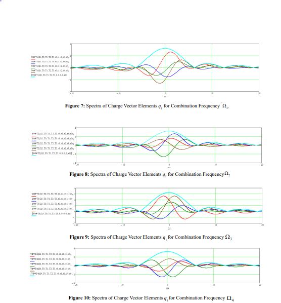
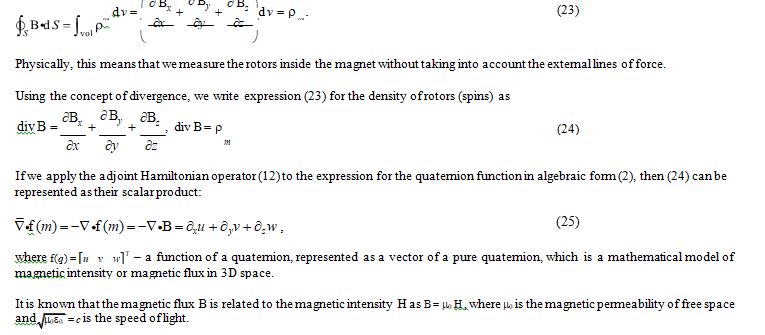
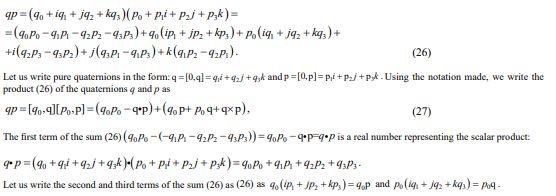
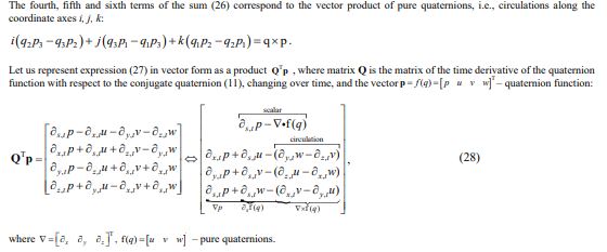
Figures 7–10 show the spectra of a three-frequency quaternion in the form of rectangular pulses of a 4D charge q1 = [5  -2  -3  2]^T, with the rectangular pulses shifted by half the duration to the right so that the beginning of the pulses coincides with zero [6]. The spectrum of the 1st vector element is shown in red, the 2nd in blue, the 3rd in green, and the 4th in brown. The turquoise color shows the modulus of the vector of spectra of rectangular pulses symmetrical to 0. As can be seen from the graphs, the
spectra of pulses shifted in time by half the pulse duration differ from the sin(x)/x function for the spectra of pulses symmetrical to 0.

The spectra in Figures 7-10 show how the magnitude of the scalar part of the electron (red lines) and the magnitude of the imaginary parts (blue, green and brown lines) change depending on the change in combination frequencies (18): Parseval's equality holds for quaternion spectra.W1, W2, W3, W4. Note that Parseval's equality holds for quaternion spectra.

Thus, an electric charge, when using a quaternion-based hypercomplex model, is represented by a 4D vector in the quaternion energy space, in which the first element is a scalar and the other three are vectors on imaginary spatial coordinates i, j, k or in matrix representation on I, J, K. Gauss's law defines charge density through the divergence of electric flux and shows how electric fields form a charge in the form of a scalar.
The time evolution of the charge vector values is represented by a dynamic model in state space, where the STM corresponds to the complex Hamiltonian operator. It is shown that an electron can perform quantum jumps with conservation of energy or rotate infinitely in an orbit with a constant radius in 4D. When using a three-frequency quaternion, the rotation orbit becomes more complex. Using the Cauchy-Riemann conditions, the linearity of the model allows us to obtain conditions that correspond to the law of conservation of energy and the principle of superposition.

The solution to the state-space dynamics equation, which is a linear homogeneous differential equation with constant coefficients, will be an exponential raised to the STM power. Since the charge model is based on a hypercomplex signal, then according to Euler's formula, hypercomplex numbers are represented in the form of harmonic functions sine and cosine with angular frequencies changing over time in a coordinate system with one real axis corresponding to the magnitude of the charge and with three imaginary (spatial) axes corresponding to the electric flow.

It is shown that using the quaternion Fourier transform it is possible to establish a connection between the magnitude of the charge elements and the value of the amplitudes and phases of the harmonics that form them, i.e., to find the frequency spectra of the charge vector elements. According to Parseval's equality for the quaternion Fourier transform, the charge value of the 4D electron vector is equal to the energy value of the harmonic functions of their generators.

 Quaternion Magnetostatic Equations
Faraday introduced the concept of magnetic flux and used lines in space to visualize the magnetic field. He called these lines flux lines or lines of force, which show the direction of magnetic field strength at each point in space. In an electric field, it is clear that the electric flow is formed by particles that have charges and are called electrons. By analogy, we can say that the magnetic flux consists of particles, which we will call rotors.

As is known, the electron has spin, which is a form of angular momentum and is its fundamental property, like charge. Therefore, the electron acts as a charge in electrical interaction and as a rotor in magnetic interaction. The circulating current (rotor) creates a magnetic field. Each rotor produces magnetic intensity. Just like the charge, the angular velocity of the rotor ω can be either positive or negative and have different values. Opposite rotors attract each other, while negative rotors repel each other. Therefore, by analogy, the angular velocity ±ω can be called the “magnetic charge”.

According to Ampere's hypothesis, a magnet consists of many elementary magnetic rotors oriented in one direction. The magnet must be considered in vector space, since its magnetism depends on its location relative to the coordinate axes in 3D. The magnetic field vector starts at the center of the rotor and is perpendicular to it. Rotors with different directions of rotation are attracted to each other, forming a scalar. In this case, the imaginary components are compensated and the poles of the connected magnets disappear, forming a large magnet also with two poles.

Thus, an electron, which has an electric charge, is a scalar particle and forms charged bodies whose intensity is the same in all directions; a rotor is a vector particle and forms magnetic bodies whose intensity is perpendicular to the radius of rotation of the circulating currents. An electron, due to duality, manifests itself as a charge during electrical interaction, and as a rotor during magnetic interaction. A magnetic field can arise when an electric field circulates. The magnetic field of a coil is made up of the magnetic fields of individual turns. Electric flux is the flow of electron charges. Magnetic flux is the flow of electron spins (rotors).

In the classical theory of electromagnetism, it is stated that the lines of magnetic flux are closed and do not end at magnetic charges, since they do not exist, therefore   . However, there is magnetic intensity and magnetic flux. Magnetic intensity and magnetic flux indicate the presence of rotors.

To measure the magnetic field strength, consider the following experiment. We drill a hole in the middle of a relatively large magnet and place it on an axis so that it rotates freely with almost no friction or inertia. We use the magnetic needle of a small compass as a point magnet. We will move the small compass to different points on the plane. The large magnet and the compass needle will rotate so that the opposite poles of the magnet and the needle point towards each other. That is, the compass needle will be affected by the force of the magnetic field of a large magnet. According to the Biot-Savart-Laplace law, the magnitude of the force will be the same on a circle whose center is located at the center of a large magnet.

This experiment is similar to the experiment with a large electric charge and with a point electric charge when measuring electrical intensity, which confirms Coulomb's law for charges. In the case of magnetic intensity, the Biot-Savart-Laplace law has a mathematical expression for magnetic intensity similar to Coulomb's law. Both show an inverse relationship with the square of the distance and a linear relationship between source and field. The difference between the experiment with charges and the experiment with magnets is that the charge is a scalar quantity and its intensity manifests itself equally in all directions without rotation of the charge. The effect of magnetic force depends on the orientation of the magnet, so to maximize the effect of magnetic force, the magnet must be turned with the corresponding pole towards the location of the point magnet.

If we consider the electron spin as a source of magnetic tension, then the rotation of the spin occurs without mechanical movement and without inertia. Since the spins of the electrons that form the large magnet are always oriented toward the location of the point magnet, it is possible to use Gauss's law to determine the density of spins pm or rotors in the magnet from the magnetic flux vector. This means that the total magnetic flux through an arbitrary closed surface with electrons creating a spin flux is equal to the closed circulating current, i.e., the rotor or spin:

In contrast to expression (21), the rotor is determined by the magnetic field strength H or magnetic flux B and shows how the magnetic flux forms the magnetic particle rotor (spin). It is known that when an electron moves in a magnetic field, it is affected by the Lorentz force, which makes it rotate. When modeling an electric field or a magnetic field using quaternions, we will have expressions (21) and (25) of the same form for the densities pq and pm . Accordingly, CRC (22) will also be valid for magnetic intensities. In addition, it will be possible to find spectra of 4D rotor vectors with different forms of amplitude changes over time and density in 4D space, similar to those presented in Figures 7–10.

 Quaternion Electrodynamic Equations
The product of quaternions in algebraic representation is calculated as [4]

In expression (28), the notations for time derivatives retain the indices denoting the coordinate axes s, x, y, z in the matrix representation and showing that time derivatives are taken from complex functions. In the representations of functions from the quaternion p, u, v, w, time indices are absent and are implied by default. It is also necessary to remember that f (q) is a function of time.

In the resulting vector (28), instead of a function of a quaternion f (q) and, accordingly, a pure quaternion f (q) , one can use the vectors
of electric E or magnetic intensity H as quaternions or as pure quaternions E and H. For the electrical intensity E or the electrical flux D, expression (28) is represented as

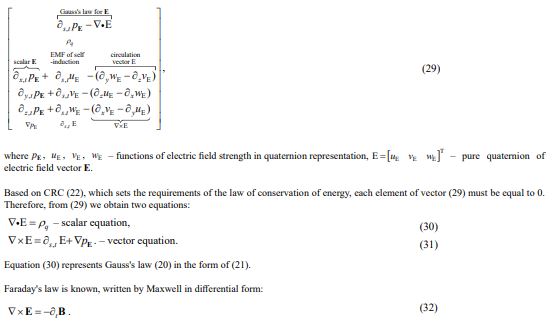
Law (32) is usually explained as follows: the change in magnetic field B over time creates an electromotive force (EMF). EMF is considered induced because magnetic flux is involved in its creation. EMF is simply the voltage that produces current in a closed circuit. The minus sign in (32) shows that the EMF is in such a direction that the created current, whose magnetic flux is added to the original flux, reduces the magnitude of the magnetic flux. The statement that the induced voltage acts to oppose the change in magnetic flux is known as Lenz's law.

In the resulting representation (31), instead of the time-varying magnetic flux ï?¶t B, EMF  Ã¯?¶s,t E is written, which creates a current in a closed circuit. As can be seen from expression (31), EMF ï?¶s,t E is proportional to circulation ï?? ï?´ E and is subtracted from it to obtain zero energy increment. In expression (31), in contrast to Maxwell’s equation, there is an additional term ï??pE – the vector of derivatives of the scalar part of the electrical field strength along the imaginary coordinate axes in matrix representation. This is explained by the fact that Maxwell's equations are written for 3D space and, when represented in quaternion form, do not take into account the scalar part. The increment of the scalar part of the field strength vector along the imaginary coordinates, together with the increment of the electric field strength vector of the imaginary part, must compensate for the increment of circulation so that their sum is equal to zero, and the energy of the electric field strength vector in the quaternion representation is preserved.

For magnetic intensity H or magnetic flux B, expression (28) takes the form:

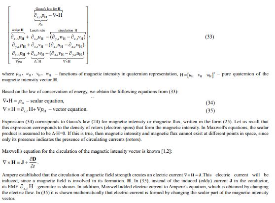
Thus, expressions for Maxwell's equations for a quaternion are obtained using the Cauchy-Riemann conditions. Basically, the resulting equations are similar to Maxwell's equations except for the presence of additional terms associated with the scalar part of the quaternion.

Conclusion

The equations of electrodynamics are obtained mathematically using the Cauchy-Riemann conditions for the quaternion. The equations represent two systems of equations for electric and magnetic intensity. The equations are identical in form and consist of an equation for the scalar part and an equation for the vector 3D part. The scalar part of the system of equations for electrical field strength corresponds to Gauss's law for charge. The scalar part of the system of equations for magnetic intensity also corresponds to Gauss's law, in which the electron spin is considered as a scalar. The representation of a quaternion in 4D space with three spatial frequencies is consistent with M. Planck's hypothesis about quantum radiation and absorption of energy of elementary particles and its dependence on frequency.

The equations obtained mathematically for the vector parts of the quaternion basically correspond to Maxwell's equations for the circulation of electric and magnetic intensities, obtained on the basis of the experiments of Faraday and Ampere. The difference is that instead of induced (eddy) currents formed by electrical and magnetic intensities, electromotive forces created by these intensities are used. In addition, the resulting equations contain currents created by the scalar parts of the quaternion. As is known, Maxwell artificially, without relying on physical experiments, added a current formed by the change in electric flow over time to the equation of circulation of magnetic intensity. This fact confirms the necessity of a quaternion model in 4D space with a scalar coordinate in electrodynamics. Since the equations of electrodynamics are obtained using linear functions of the quaternion, these functions are also the solution of these equations.

References

1.    Hayt, W., & Buck, J. (2012). Engineering electromagnetics.
2.    Fleisch, D. (2008). A student's guide to Maxwell's equations. Cambridge University Press.
3.    Kantor, I. L., Solodovnikov, A. S., & Shenitzer, A. (1989). Hypercomplex numbers: an elementary introduction to algebras (Vol. 302). New York: Springer-Verlag.
4.    Morais, J. P., Georgiev, S., & Sprößig, W. (2014). Real quaternionic calculus handbook.
5.    Sovetov, V. (2024). The MIMO data transfer line with three-frequency quaternion carrier. Journal of Sensor Networks and Data Communications, 4(2), 01-17.
6.    Sovetov, V. (2024). Three-Frequency Quaternion Fourier Transform. J Res Edu, 2(2), 01-13.