Leveraging Econometric and Deep Learning Methods for Comprehensive Analysis of Global Equity Market Returns and Volatility

Introduction

The global market refers to the interconnected network of economies, industries, and financial systems that span across borders, facilitating the exchange of goods, services, capital, and investments. It is driven by factors such as international trade, capital flows, and geopolitical dynamics, making it essential for investors, policymakers, and analysts to understand its behaviour. Analysing the global market helps stakeholders identify trends, assess risks, and make informed decisions, especially when dealing with diverse asset classes and international investments. Given the complexity and volatility of these markets, researchers employ various statistical and computational models to capture the intricate relationships and forecast future market movements.

The primary focus in global market analysis is the study of equity indices, which serve as barometers for market performance. These indices, such as the MSCI World Index and the iShares MSCI ACWI ETF, are used to track the performance of large segments of the global equity market. The MSCI World Index represents developed markets, while the ACWI ETF provides exposure to both developed and emerging markets, offering a more comprehensive view of the global economy. Understanding the behaviour of these indices is crucial for investors who seek to diversify their portfolios and optimize returns while managing risk. To analyse the relationship between these indices and their volatility, researchers employ various advanced models. The Vector Autoregressive (VAR) model examines the dynamic interdependencies between multiple time series, allowing researchers to explore how one index influences another over time, identifying lead-lag relationships. The Bayesian model provides a probabilistic framework that incorporates uncertainty and prior knowledge, offering a more flexible approach to parameter estimation, especially when data is sparse or noisy. GARCH (Generalized Autoregressive Conditional Heteroskedasticity) models are widely used to model and forecast volatility, a crucial component of market risk. These models are designed to capture time-varying volatility, which is essential for understanding how market risk evolves, particularly during periods of economic stress.

This study focuses on the MSCI World Index and the iShares MSCI ACWI ETF, two major global equity indices, to explore their return dynamics and volatility patterns. By applying these advanced models, the research aims to uncover deeper insights into the relationship between these indices and the broader global market, providing valuable information for investors and analysts seeking to navigate the complexities of global financial markets.

Literature Review

According to tree-based models and neural networks to predict stock market group values in the Tehran Stock Exchange, focusing on 1 to 30-day forecasts. Among all models, LSTM outperformed others with the lowest error rates and best fit, though its runtime was significant. The research suggests potential for these algorithms in stock prediction, recommending further exploration on other markets and hyperparameter effects [1].

According to explored conventional, machine learning, and deep learning techniques for stock market forecasting, highlighting recent applications and ensemble models on specific stock datasets [2]. Despite the variety of methods available, no universal solution exists for accurately predicting stock prices, as AI models can fail without efficient training on fresh data. The authors emphasize the need for hyperparameter tuning to improve prediction accuracy and suggest using AI models as supplementary tools for traders and advisors. Future research should focus on portfolio management, trading strategies, and investment decision-making alongside stock forecasting.

Demonstrated his survey with many articles in between 2017 to 2019 to summarize recent progress in deep learning–based stock market prediction, covering data collection, processing, modelling, and evaluation the authors emphasize implementation details and reproducibility to support adopting published models as baselines. Their insights and identified future directions aim to accelerate and guide further research in the field [3].

According to financial time series forecasting using deep learning and technical analysis, focusing on predictor techniques, trading strategies, profitability metrics, and risk management [4]. They found LSTM to be the most widely used model due to its memory capabilities, with hybrid models showing promising results. However, only a minority of studies assessed profitability and even fewer addressed risk management, despite their importance. The authors highlight several research gaps, including advanced trading strategies, hybrid qualitative–quantitative models, and better links between performance and profitability. demonstrated in their research article that integrating with deep learning improves stock-chart prediction accuracy over conventional neural networks, with optimal performance at a window size of 20 and a dimension; their results show that DNNs outperform RBFNNs (Radial Basis Function Neural Network) and RNNs in hit-rate and return-correlation accuracy, though they lag in Total Return and RMSE, and they suggest that future work using advanced deep-learning techniques could further enhance performance and extend applications to portfolio management and trading strategies [5]. proposed two methods for predicting stock indices and prices, beginning with a FFNN (Feed-forward Neural Network) that achieves 97.66% accuracy but requires extensive training and regularisation to address overfitting. They then introduce a CNN (Convolution Neural Network) model using greyscale 2-D histograms of time-series segments, which reduces training time and data requirements while improving accuracy to 98.92%. Although generating synthetic histogram images adds computational overhead, the CNN approach proves more efficient overall. Both methods deliver highly accurate predictions, offering valuable tools for analysts aiming to forecast stock-market trends [6].

Presented an RCNN (Region-based Convolutional Neural Network) model that integrates news titles and technical indicators, outperforming standard CNNs by capturing both local and temporal patterns [7]. They showed that using only prior-day news yields superior forecasts, indicating that news has a short-lived impact on markets and that sentence embeddings work better than word embeddings for this task. The authors propose future work using stronger embedding methods and reinforcement learning to develop trading strategies that focus on significant price movements.

Evaluate four deep-learning models (MLP, RNN, LSTM, CNN) on NSE and NYSE stocks, showing they can learn common underlying market dynamics across both exchanges. Their results demonstrate that all DL models outperform the linear ARIMA baseline, with CNN performing best due to its ability to capture abrupt changes through windowed inputs. They note that hybrid architectures were not explored and could offer further improvements in future work [8]. According to machine-learning methods can substantially enhance financial-market prediction by uncovering complex patterns in historical data, leading to more informed decisions and potentially higher returns with lower volatility [9]. The study emphasises that model choice and hyperparameter tuning are critical, as performance varies with data structure, market conditions, and asset characteristics. It recommends future comparative research across models and environments to further strengthen real-time predictive decision-making in evolving economic settings.

Research Methodology

In this section, it outlines the methodological framework employed to analyse the return and volatility dynamics of the MSCI World Index and the iShares MSCI ACWI ETF. A combination of statistical, econometric, and deep learning models has been utilised to capture linear relationships, dynamic interactions, volatility patterns, and nonlinear forecasting behaviour. Financial time series exhibit characteristics such as heavy tails, volatility clustering, asymmetric responses to shocks, and weak predictability; therefore, a multi-method approach is essential for obtaining robust insights. The methodology is divided into descriptive analysis, regression modelling, vector autoregression, volatility modelling, and deep learning techniques, each selected to address specific features of market behaviour.

Descriptive Statistical Analysis

Descriptive statistics are used as an initial step to summarise the distributional characteristics of MSCI and ACWI returns before advanced modelling. They provide insight into the central tendency, variability, and dispersion of the data and help identify potential anomalies, heavy-tailed behaviour, or clustering in returns. These measures include the mean, variance, standard deviation, quartiles, and range.

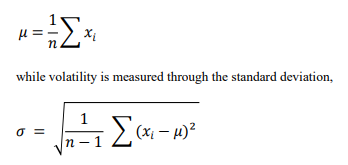
Summary statistics allows comparison of the risk-return characteristics of MSCI and ACWI and reveals which index exhibits greater fluctuation. Visual tools such as histograms and boxplots further assist in identifying symmetry, kurtosis, and the presence of extreme values.

Linear Regression Modelling (OLS and Bayesian Regression)

Linear regression is a statistical method used to model the linear relationship between a dependent variable and one or more independent variables by fitting a straight line to the observed data, primarily for prediction and analysis.

Ordinary Least Squares (OLS)

OLS regression is applied to evaluate the linear relationship between MSCI and ACWI returns. This model determines whether MSCI provides predictive information for ACWI based on the slope coefficient. The OLS model is specified as:

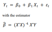
This analysis helps quantify the sensitivity of ACWI to MSCI and determines whether the two indices move proportionally or exhibit structural differences.

Bayesian Regression

Bayesian regression is implemented to account for uncertainty in parameter estimation, which is especially important in volatile financial environments. Unlike OLS, which produces point estimates, Bayesian regression incorporates prior beliefs and provides posterior distributions for regression parameters:

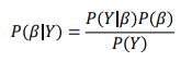
Posterior credible intervals allow more robust statistical inference. This method is used to validate OLS results while quantifying the uncertainty surrounding the relationship between MCSI and ACWI.

Vector Autoregressive Models (VAR and Bayesian VAR)

VAR (Vector Autoregression) is important because it is a flexible, atheoretical model that simultaneously captures and forecasts the complex, dynamic interdependencies among multiple related time series variables.

VAR Model

A Vector Autoregression (VAR) framework is employed to capture dynamic interdependencies between MSCI and ACWI across multiple time lags. Since financial indices often influence one another, VAR treats both MSCI and ACWI as endogenous variables:

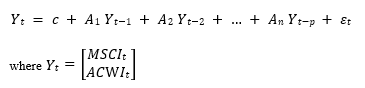
This model identifies lead–lag relations, directional causality, and how shocks propagate across global markets.

Bayesian VAR

To improve estimation reliability and prevent overfitting, the Bayesian VAR model is implemented:

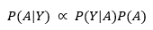
BVAR stabilises the estimation of dynamic parameters and provides credible intervals, ensuring robust inference.

Volatility Modelling (GARCH Family Models)

ARCH (Autoregressive Conditional Heteroscedasticity) is a time series model where the variance of the error term at current time period, which is a function of the squared error terms from previous periods, and its importance lies in being the first model to successfully capture and formally quantify volatility clustering in financial data, changes in daily price tend to be followed by fluctuations in daily return, while GARCH (Generalized Autoregressive Conditional Heteroscedasticity) enhances this by allowing the current conditional variance to also depend on lagged conditional variances, providing a much more parsimonious and realistic model for modelling the persistence of volatility over time.

GARCH Model

'GARCH (1,1) is often used as the default in this paper, parsimonious model for each univariate volatility of change in stock prices within a broader Multivariate GARCH framework because it effectively captures volatility clustering with only three parameters, which is a crucial first step for subsequently modelling the correlation between the two stocks. The GARCH (1,1) model is used to capture volatility clustering as,

It assesses how markets absorb shocks and measures the persistence of volatility.

EGARCH Model

The EGARCH model captures asymmetric volatility responses

It identifies leverage effects where negative shocks increase volatility more than positive shocks.

GJR-GARCH Model

The GJR-GARCH specification captures threshold asymmetry

It tests whether downside shocks produce disproportionate volatility

Deep Learning Models (RNN, LSTM, DNN, and BNN)

Deep learning is vital in stock market analysis because its models, like LSTM and GRU networks, can automatically extract complex, non-linear patterns from vast amounts of both structured and unstructured data to provide more accurate and adaptive forecasts of future price movements than traditional statistical methods

Recurrent Neural Network (RNN)

RNNs model sequential dependencies:

They capture short-term temporal patterns in financial returns. Additional Note: RNNs are effective when data exhibit short memory, and their recurrent structure makes them suitable for modelling basic temporal dependencies. However, they often struggle with long sequences due to vanishing gradients, motivating the need for more advanced architectures.

Long Short-Term Memory (LSTM)

LSTMs handle long-term dependencies using gating mechanisms:

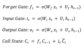
They outperform RNNs in modelling nonlinear return dynamics. LSTMs are particularly suitable for financial markets because they can recognise long-range patterns and structural breaks. Their memory cells help retain information through turbulent market periods, improving forecasting stability.

Deep Neural Network (DNN)

DNNs learn nonlinear relationships through multiple hidden layers:

They provide a non-sequential baseline comparison. DNNs allow the extraction of complex feature representations, which can capture nonlinear transformations in financial data. However, they lack memory mechanisms, making them less effective for time-series forecasting relative to RNNs and LSTMs.

Bayesian Neural Network (BNN)

BNNs incorporate predictive uncertainty

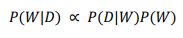
They generate confidence intervals, useful under market volatility. BNNs are particularly advantageous in finance because uncertainty quantification is essential for risk assessment. Their probabilistic nature helps identify periods of high uncertainty, improving interpretability during extreme market conditions.

Volatility Estimation Measures (Realized and Parkinson Volatility)

Volatility Estimation Measures are crucial in financial stock prices because it can provide the quantitative measure of risk necessary for risk management, derivatives pricing, and optimal portfolio allocation decisions

Realized Volatility

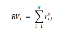
This model captures high-frequency market variability. Realized volatility effectively reflects true market movements by including intraday variations, making it highly responsive to sudden shocks. It is valuable for comparing model-generated volatility to actual market behaviour.

Parkinson Volatility

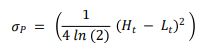
This model provides a smoother volatility estimate using high–low price ranges. Parkinson volatility is more efficient than close-to-close volatility estimators because it uses additional price information. It is especially useful for long-term volatility tracking where extreme short-term noise must be minimized.

Data Analysis and Results

The dataset has been collected from Investing India website. In this dataset global two stocks have been chosen, MSCI WORLD INDEX and iShares MSCI ACWI ETF. In this paper data has been collected from 01-04-2020 to 17-11-2025. There are total number of 1477 entries. It is a daily based dataset on daily returns. Descriptive statistics has been provided below to better understanding of the dataset.

Descriptive Statistics	MSCI Return	ACWI Return
count	1477	1477
mean	0.000006	0.000006
std	0.000095	0.000089
min	-0.000584	-0.000537
25%	-0.000039	-0.000037
50%	0.000008	0.000008
75%	0.000056	0.000052
max	0.000647	0.00057

Table:1 Summary Statistics

In Table-1, descriptive statistical assessment has been conducted to compare the performance characteristics of the MSCI Return and ACWI Return series, based on 1,477 daily observations for each index, in order to identify differences in their return distribution and risk exposure. The mean daily returns for both indices were found to be identical at approximately 0.000006, indicating that the average performance of global equity exposure was captured similarly by each benchmark over the period analysed. However, distinctions emerged when volatility and dispersion metrics were examined. The MSCI index exhibited a slightly higher standard deviation (0.000095) compared to ACWI (0.000089), suggesting that MSCI returns were subject to moderately higher fluctuations and thus reflected marginally greater risk. This finding was reinforced by a wider return range observed in MSCI, with minimum and maximum returns at −0.000584 and 0.000647 respectively, exceeding the narrower range of ACWI between −0.000537 and 0.000570, which indicated greater susceptibility of MSCI to extreme market movements. Quartile-based evaluations further demonstrated that the MSCI index showed slightly lower returns in the bottom quartile and slightly higher returns in the upper quartile relative to ACWI, implying broader variability and a marginally heavier tail structure on both downside and upside distribution segments. Despite these differences, the median values for both indices were perfectly aligned at 0.000008, signalling that their central tendency and typical return behaviour remained nearly indistinguishable. Overall, this statistical profile confirmed that MSCI and ACWI are highly aligned in representing global equity returns, while still revealing that MSCI may involve a marginally higher volatility risk but also slightly enhanced upside potential, offering useful insight for investors considering the balance between return consistency and tolerance for market variability.'

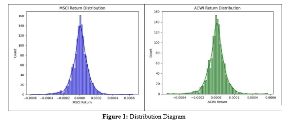
The distribution histograms for MSCI and ACWI returns reveal that both indices exhibit a highly peaked, leptokurtic shape cantered near zero, indicating that most daily returns cluster tightly around the mean. The tails on both sides extend noticeably, suggesting the presence of occasional extreme return events and non-normal behaviour. MSCI demonstrates slightly wider dispersion compared to ACWI, consistent with its marginally higher volatility. Despite these differences, the overall symmetry and strong concentration around zero highlight the similar risk-return characteristics shared by the two globally diversified indices.

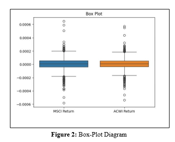
The box plot shows that both MSCI and ACWI returns are tightly cantered around zero, indicating similar median performance. However, MSCI exhibits greater spread in the interquartile range, along with more extreme outliers on both ends, suggesting slightly higher volatility and exposure to tail risk. ACWI appears more compact and stable by comparison, reflecting marginally lower variability in daily return movement.

	coefficient	σ	error	t-statistics
constant	5.30E-06	2.31E-06	2.294	0.022
MSCI Return	0.112	0.024	4.608	0

Omnibus:	154.158	Durbin-Watson:	1.996
P(Omnibus):	0.003	Jarque-Bera (JB)	1207.261
Skew:	-0.017	P(JB):	7.02E-263
Kurtosis:	7.429	Cond. No	1.05E+04

                                                                           Table 3: OLS Regression Output

The OLS regression analysis indicates a statistically significant positive relationship between MSCI returns and ACWI returns, with the MSCI coefficient recorded as 0.112 and a p-value less than 0.05, suggesting that changes in MSCI returns contribute positively to the prediction of ACWI returns. However, the explanatory power of the model remains very low, as shown by the R-squared value of only 0.014, meaning that just 1.4% of the variation in ACWI returns is explained by MSCI returns alone. This reveals that while the indices move together directionally, additional market factors drive ACWI performance beyond what MSCI captures. The Durbin-Watson statistic of 1.996 indicates limited autocorrelation concerns, supporting reliability in regression structure. Nevertheless, residual diagnostics show non-normality through a high Jarque-Bera statistic, negative skewness, and a kurtosis value of 7.429, reflecting heavy-tailed behaviour and potential volatility clustering in the return data. These findings highlight that although the relationship is statistically significant, the model lacks strong predictive capability and requires expansion with more explanatory variables or advanced modelling methods for improved forecasting accuracy.

	μ	σ	hdi3%	hdi97%	mcseμ	mcseσ	essbulk	esstail	r^
α	0	0	0	0	0	0	6328	3092	1
β	0.112	0.023	0.067	0.154	0	0	5852	3072	1
σ	0	0	0	0	0	0	6690	2450	1

Table 4: Bayseian Regression Output

The Bayesian regression analysis reinforces the findings observed in the classical OLS model, while providing more robust uncertainty quantification. The posterior mean estimated for the beta coefficient is 0.112, closely matching the OLS coefficient, indicating a consistent positive relationship between MSCI returns and ACWI returns. The 94% Highest Density Interval (HDI) ranges from 0.067 to 0.154, which does not cross zero, confirming the statistical significance of the relationship in the Bayesian framework as well. The alpha (intercept) is centred at zero with a very narrow uncertainty range, implying negligible constant bias between the two indices. The sigma parameter shows very low posterior uncertainty, reflecting stable residual variance despite volatility clusters identified previously. Essential metrics such as ESS (Effective Sample Size) indicate high reliability in sampling for both bulk and tail distributions, and the value of 1 confirms excellent convergence of Markov Chain Monte Carlo estimations. Overall, Bayesian modelling validates that MSCI returns are a credible predictor of ACWI movements, but the modest magnitude of beta still suggests limited explanatory power. This confirms the need for inclusion of additional predictors or nonlinear models to capture broader market dynamics more effectively.

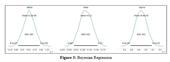
Figure-3 displays posterior distributions for the Bayesian regression parameters alpha, beta, and sigma. Alpha is centred extremely close to zero with a narrow 94% HDI, indicating almost no constant bias. Beta, with a mean around 0.11 and an HDI from roughly 0.067 to 0.15, confirms a positive and statistically credible relationship between MSCI and ACWI returns. Fluctuation of values showing tightly bounded residual volatility. All three parameters exhibit smooth, well-behaved posterior shapes and strong convergence, reinforcing the reliability of the Bayesian estimates.

No. of Equations	2	BIC:		-41.7072
Nobs:	1475	HQIC:		-41.7297
Log-Likelihood	26609.7	FPE:		7.43E-19
AIC:	-41.7431	Det(ωmle):		7.38E-19
Results for equation MSCI Return	coefficient	std. error	t-stat	prob
const	0	0	1.263	0.207
L1.MSCI Return	-0.13969	0.025892	-5.395	0
L1.ACWI Return	1.058454	0.002871	368.662	0
L2.MSCI Return	-0.00939	0.002934	-3.201	0.001
L2.ACWI Return	0.100766	0.02752	3.661	0
Results for equation ACWI Return	coefficient	std. error	t-stat	prob
const	0.000005	0.000002	2.371	0.018
L1.MSCI	0.468546	0.234506	1.998	0.046
L1.ACWI	0.120855	0.026003	4.648	0
L2.MSCI	-0.04724	0.02657	-1.778	0.075
L2.ACWI	-0.47896	0.24925	-1.922	0.055

Correlation matrix of residuals	MSCI Return	ACWI Return
MSCI Return	1	0.042368
ACWI Return	0.042368	1

Table 5: VAR-OLS Model

The above analytical outcome in Table-5 shows that both indices exhibit very similar average performance and highly concentrated distributions around zero. Despite this resemblance, MSCI demonstrates slightly higher volatility and broader tails, indicating greater exposure to extreme return movements on both the upside and downside. Visual tools such as boxplots, histograms, and summary statistics consistently highlight this pattern, even though the overall central tendencies of the two indices remain closely aligned, reflecting their shared role as global equity benchmarks.

This OLS model in Table-5 identifies a positive and statistically significant effect of MSCI on ACWI returns; however, the extremely low value reveals that MSCI explains only a minimal share of ACWI’s variation. Diagnostic tests confirm typical financial characteristics such as non-normality and heavy-tailed behaviour. Bayesian regression supports the OLS findings, with nearly identical parameter estimates and credible intervals that affirm a modest but reliable relationship. These results collectively indicate that MSCI offers some predictive information but is insufficient for fully capturing global return dynamics on its own. This OLS-VAR model emerges from the VAR (2) model, which reveals an asymmetric dynamic linkage. ACWI has a substantially stronger effect on MSCI, suggesting that global market movements captured by ACWI influence MSCI with greater intensity than the reverse. Meanwhile, MSCI exerts only moderate feedback on ACWI. Both indices exhibit short-term continuation and two-day mean reversion, features commonly observed in financial time series. The low residual correlation demonstrates the effectiveness of OLS-VAR model in capturing joint patterns. Overall, the findings underscore that ACWI serves as the broader global driver, while MSCI reacts more sensitively to global shocks for highlighting the value of multi-index modelling for understanding interconnected market behaviour.

	μ	σ	hdi3%	hdi97%	mcseμ	mcseσ	essbulk	esstail	r^
a1	0	0	0	0	0	0	6517	4554	1
a2	0	0	0	0	0	0	6222	3897	1
b11	0.118	0.026	0.071	0.169	0	0	5972	4110	1
b12	0.02	0.025	-0.026	0.066	0	0	5963	4122	1
b21	1.058	0.003	1.052	1.063	0	0	6641	4452	1
b22	-0.045	0.003	-0.05	-0.04	0	0	6756	4670	1
σ1	0	0	0	0	0	0	6820	4519	1
σ1	0	0	0	0	0	0	6303	4239	1

Table 6: Bayesian VAR Model

The Bayesian VAR parameter estimates reveal a clear and well-identified dynamic relationship between MSCI and ACWI returns. The intercept terms (a1 and a2) are effectively zero with extremely narrow uncertainty ranges, indicating no constant bias in either equation. The own-lag effect of MSCI on itself (b11) is positive mean (μ ≈ 0.118) with an HDI that excludes zero, demonstrating mild return persistence, while the cross-lag from ACWI to MSCI (b21) is very strong mean (μ ≈ 1.058) and tightly estimated, confirming that ACWI has a dominant influence on subsequent MSCI movements. In contrast, the effect of MSCI on ACWI is weak: the cross-lag coefficient (b12) has an HDI that includes zero, indicating no credible influence, whereas ACWI own-lag (b22) is small and negative, suggesting slight mean reversion. All parameters show high effective sample sizes and convergence diagnostics (r^ = 1), reflecting excellent MCMC stability. Overall, the results affirm an asymmetric relationship where ACWI drives MSCI strongly, while MSCI provides only limited predictive information for ACWI.

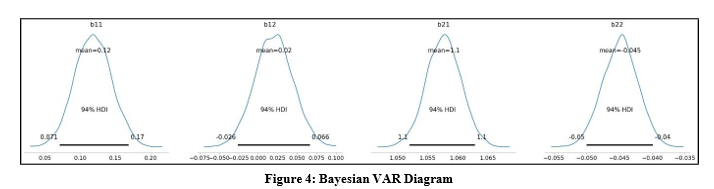
In Figure-4, the posterior density plots for the VAR coefficients clearly illustrate the asymmetric dynamic relationship between MSCI and ACWI returns. The b11 coefficient (MSCI own lag) has a positive mean around 0.12, with its entire 94% HDI lying above zero, indicating credible short-term persistence in MSCI returns. In contrast, b11 (ACWI effect on MSCI) has a small mean near 0.02 and an HDI that spans both negative and positive values, showing that ACWI does not exert a statistically reliable influence on MSCI in this equation. The most pronounced effect appears in b21, where ACWI responds strongly to MSCI’s past movements: the posterior is sharply peaked around 1.1 with an extremely narrow HDI fully above one, confirming that MSCI has a dominant and highly credible impact on ACWI within the VAR structure. Meanwhile, b22 shows a small negative mean (approximately –0.045) with an HDI entirely below zero, indicating mild mean reversion in ACWI returns. Therefore, these posterior distributions indicating that MSCI exerts a strong and consistent influence on ACWI, while ACWI have direct impact on MSCI is weak and statistically uncertain, reinforcing an asymmetric causal structure in return dynamics.

GARCH	β1	0.88	2.37E-02	37.078	6.46E-301
EGARCH	μ	7.20E-04	1.98E-04	3.632	2.81E-04
EGARCH	ω	-0.355	0.16	-2.224	2.61E-02
EGARCH	α1	0.2083	5.80E-02	3.594	3.25E-04
EGARCH	β1	0.9623	1.68E-02	57.302	0.001
GJR-GARCH	μ	9.17E-04	2.45E-04	3.736	1.87E-04
GJR-GARCH	ω	1.78E-04	1.44E-03	0.124	0.901
GJR-GARCH	α1	0.01	0.243	0.04113	0.967
GJR-GARCH	γ1	0.05	6.39E-02	0.783	0.434
GJR-GARCH	β1	0.945	0.393	2.407	1.61E-02

Table 7: GARCH Family Model

The GARCH-family results indicate that volatility in the return series exhibits strong persistence, asymmetric effects, and varying levels of explanatory power across models. The standard GARCH (1,1) model shows statistically significant parameters, with α₁ = 0.10 and β₁ = 0.88, both highly significant, confirming that past shocks and past volatility strongly influence current volatility. The large sum (α1 + β₁ ≈ 0.98) indicates extremely persistent volatility— typical of financial return series—with shocks decaying very slowly over time. The EGARCH model provides additional insight by capturing asymmetry: both α1 and β1 are significant, while the negative and significant parameter (ω) suggests a leverage effect, meaning negative shocks disproportionately increase volatility more than positive shocks. This reflects the common phenomenon that markets react more strongly to downturns than upswings. The GJR-GARCH model, however, performs relatively weakly— only β₁ is statistically significant, while α₁,γ₁, and ω have high p − values, implying that neither standard shocks nor asymmetric effects are strongly supported in this specification. This suggests that the data does not generate strong threshold-type asymmetric volatility captured by the GJR structure. Overall, the GARCH and EGARCH models provide statistically robust evidence of persistent and asymmetric volatility dynamics, while the GJR-GARCH model offers limited additional explanatory power, indicating that smooth asymmetric responses EGARCH may better describe the volatility behaviour of the return series than threshold-based mechanisms.

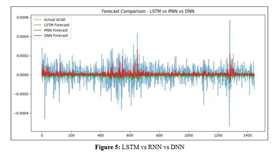
In Figure-5 the forecast comparison plot between LSTM, RNN, and DNN models against the actual ACWI returns shows that all three neural-network models struggle to fully capture the sharp fluctuations and volatility spikes present in the real data. The actual ACWI series exhibits frequent high-frequency noise and occasional extreme movements, while the model forecasts remain much smoother and closer to zero, indicating a strong bias toward predicting the mean rather than the true variability of returns. Among the models, the LSTM and RNN forecasts track the directional movements slightly better than the DNN,particularly during moderate volatility periods, reflecting their ability to incorporate temporal dependencies. However, all models significantly underreact to extreme upward or downward spikes, demonstrating that deep learning architectures have limited effectiveness in forecasting daily financial returns, which are notoriously noisy and weakly predictable. Therefore, the plot suggests that although these neural-network models provide stable and low-variance forecasts, they fail to match the amplitude and intensity of real market movements, reinforcing the fundamental difficulty of predicting short-horizon return series.

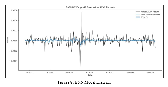
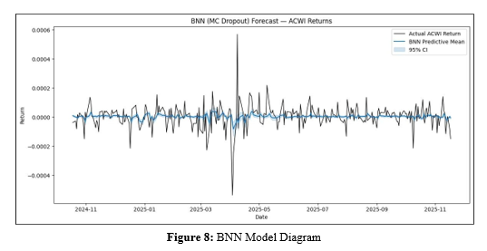
In Figure-8: the Bayesian Neural Network (BNN) forecast using Monte Carlo dropout method reveals that the model provides a smoother predictive mean compared to the actual ACWI return series, which remains highly volatile and noisy. Here the BNN model captures the general direction and low-frequency movements of returns but, similar to other neural network models, fails to replicate sharp spikes or sudden deviations that characterize real financial data. The inclusion of a 95% confidence interval is particularly valuable: the shaded uncertainty band widens modestly around periods of elevated volatility, showing that this BNN model is able to quantify predictive uncertainty more effectively than deterministic deep learning models. However, even with uncertainty estimates, the confidence interval still does not fully encompass extreme return shocks, illustrating that financial return volatility is difficult to anticipate, even probabilistically. Therefore, here the selected BNN model demonstrates improved uncertainty representation but continues to provide conservative, mean-reverting forecasts, highlighting both the strengths and limitations of Bayesian deep learning in modelling unpredictable market return dynamics.

In Figure-9, Volatilitlity Model Comparisons shows two different volatility measures: Realized Volatility and Parkinson Volatility. Realized Volatility exhibits sharper peaks and more pronounced fluctuations, capturing the actual observed variability in asset returns. This measure highlights periods of high market volatility and sudden price changes. On the other hand, Parkinson Volatility, which is based on the range between the highest and lowest prices during each period, presents a smoother pattern with less extreme spikes. This indicates a more stable view of volatility. In this scenario, Realized Volatility provides a detailed, immediate reflection of market uncertainty, Parkinson Volatility offers a broader, less reactive perspective. The comparison underscores the different ways these models capture market dynamics and their suitability for various types of volatility analysis. These differences highlight how different volatility models can provide varying insights into market dynamics.

Conclusion

In conclusion, this integrated study provides a comprehensive analysis of the risk and return dynamics between two global equity indices, the MSCI WORLD INDEX and iShares MSCI ACWI ETF, over the selected period from 1st April 1, 2020, to 17th November, 2025. The descriptive statistics reveal that both indices exhibit nearly identical average returns, but MSCI shows slightly higher volatility and a broader range of returns, indicating a marginally higher risk profile. Despite these differences in volatility, the median values for both indices are nearly identical, suggesting that their central tendencies are closely aligned [10- 14].

The regression analyses model both OLS and Bayesian Regression confirmed a positive and statistically significant relationship between MSCI and ACWI returns, but with very low explanatory power, indicating that other factors significantly drive ACWI performance. The VAR model further supports this, revealing that ACWI has a stronger influence on MSCI, while the reverse effect is more limited. These findings suggest that global market movements captured by ACWI play a more dominant role in influencing MSCI returns. The volatility modeling, through GARCH-family models, highlights the persistence of volatility and its asymmetric nature, with negative shocks leading to higher volatility. The comparison of volatility models (Realized Volatility vs. Parkinson Volatility) shows that while Realized Volatility captures more immediate market fluctuations, Parkinson Volatility provides a smoother, long-term view of volatility, highlighting the importance of selecting appropriate volatility measures based on the analysis context.

Therefore, MSCI and ACWI are closely aligned in their return behavior, the study reveals significant differences in their volatility patterns and market dynamics. These insights are crucial for investors seeking to balance return consistency with risk tolerance, and they underline the need for a multi-model approach to better understand market interdependencies.

Further Scope of the Research

In this decade, technology is evolving day by day. New machine learning algorithms are evolving to analyse the market volatility. New analytical methods of sceintific research are also inventing and innovating to develop the economy of any nation. In future there will be more advanced statistical tools, algorithms available to get accurate prediction to remove the obstacles in growing economy.

Limitations of this research

Research on financial risk may face inherent uncertainty of predicting future. Assuming variables can be fluctuating every time and may not follow the distribution models. Furthermore, the complexity in the global economy vary with different times with respect to growing technology and other variables such as nature volatility.

Ethical Standards

The research work was conducted in adherence to the highest ethical standards, with integrity and transparency. In this paper, all findings and analyses were presented with honesty and without bias or manipulation.

Funding

Author did not get any funds for this research.

Declaration of Interest

Author has no conflict of interest.

Data Sharing Statement

Data is available on Investing India website.

References

1. Nabipour, M., Nayyeri, P., Jabani, H., Mosavi, A., Salwana, E., & S, S. (2020). Deep learning for stock market prediction. Entropy, 22(8), 840.
2. Sonkavde, G., Dharrao, D. S., Bongale, A. M., Deokate, S. T., Doreswamy, D., & Bhat, S. K. (2023). Forecasting stock market prices using machine learning and deep learning models: A systematic review, performance analysis and discussion of implications. International Journal of Financial Studies, 11(3), 94.
3. Jiang, W. (2021). Applications of deep learning in stock market prediction: recent progress. Expert Systems with Applications, 184, 115537.
4. Li, A. W., & Bastos, G. S. (2020). Stock market forecasting using deep learning and technical analysis: a systematic review. IEEE access, 8, 185232-185242.
5. Singh, R., & Srivastava, S. (2017). Stock prediction using deep learning. Multimedia Tools and Applications, 76(18), 18569-18584.
6. Mukherjee, S., Sadhukhan, B., Sarkar, N., Roy, D., & De, S. (2023). Stock market prediction using deep learning algorithms. CAAI Transactions on Intelligence Technology, 8(1), 82-94.
7. Vargas, M. R., De Lima, B. S., & Evsukoff, A. G. (2017, June). Deep learning for stock market prediction from financial news articles. In 2017 IEEE international conference on computational intelligence and virtual environments for measurement systems and applications (CIVEMSA) (pp. 60-65). IEEE.
8. Hiransha, M. E. A. G., Gopalakrishnan, E. A., & Soman, K.P. (2018). NSE stock market prediction using deep-learning models. Procedia computer science, 132, 1351-1362.
9. Perumallaplli, R. (2012). Machine Learning Algorithms for Accurate  Stock  Market  Forecasting:  Case  Studies2012. Available at SSRN 5228711.
10. Ajiga, D. I., Adeleye, R. A., Tubokirifuruar, T. S., Bello, B. G., Ndubuisi, N. L., Asuzu, O. F., & Owolabi, O. R. (2024). Machine learning for stock market forecasting: a review of models and accuracy. Finance & Accounting Research Journal, 6(2), 112-124.
11. Chowdhury, M. S., Nabi, N., Rana, M. N. U., Shaima, M., Esa, H., Mitra, A., ... & Naznin, R. (2024). Deep learning models for stock market forecasting: A comprehensive comparative analysis. Journal of Business and Management Studies, 6(2), 95.
12. Liu, H., & Long, Z. (2020). An improved deep learning model for predicting stock market price time series. Digital Signal Processing, 102, 102741.
13. Liu, Q., Tao, Z., Tse, Y., & Wang, C. (2022). Stock market prediction with deep learning: The case of China. Finance Research Letters, 46, 102209.
14. Singh, S., Madan, T. K., Kumar, J., & Singh, A. K. (2019, July). Stock market forecasting using machine learning: today and tomorrow. In 2019 2nd International Conference on Intelligent Computing, Instrumentation and Control Technologies (ICICICT) (Vol. 1, pp. 738-745). IEEE.