Inventory Modelling for Restaurant’s Demand and Supply - A Case Study with Reference to a Hyderabad Restaurant’s

Introduction

Inventory management plays a pivotal role in the smooth functioning of the restaurant industry, where effective stock control is crucial to maintaining service quality and profitability. The industry faces unique challenges such as fluctuating customer demand, limited shelf life of ingredients, and the need to avoid overstocking or stockouts. These challenges require a fine balance between maintaining sufficient stock to meet customer demand and minimizing waste caused by expired products. Inefficiencies in inventory management can lead to significant financial repercussions. For instance, overstocking not only results in increased storage costs but can also cause perishable items to spoil, leading to unnecessary waste. On the other hand, understocking can result in stockouts, leading to missed sales opportunities, dissatisfied customers, and, ultimately, lost revenue. Therefore, managing inventory efficiently is essential for a restaurant's financial sustainability and operational success. This study addresses these challenges by proposing a data-driven inventory management model. The model focuses on optimizing stock levels using historical sales data and predictive algorithms to forecast future demand. By doing so, it aims to minimize inventory costs while ensuring that the restaurant can consistently meet customer demands. The study utilizes various inventory management techniques, including the Economic Order Quantity (EOQ) model, demand forecasting, and safety stock.

Importance of the Study to Society

Moreover, improving inventory practices can lead to cost sav- ings for restaurants, which This study holds significant societal value, particularly in promoting sustainability and resource effi- ciency in the food industry. Food waste is a major global issue, and the restaurant sector contributes significantly to this problem. By optimizing inventory management, restaurants can reduce waste, thereby supporting environmental sustainability. Addition- ally, efficient inventory management ensures that food resources are utilized effectively, reducing the strain on food supply chains and promoting better resource utilization. It could be passed on to customers in the form of lower prices, further enhancing the competitiveness of the restaurant industry. In a broader context, this study helps highlight how operational improvements in one sector (restaurants) can have a ripple effect on the economy, envi- ronment, and society as a whole, particularly in terms of reducing waste and improving economic efficiency.

Research Background

The motivation behind selecting this topic stems from the grow- ing need for restaurants to manage inventory more effectively. The challenges of meeting fluctuating customer demand while manag- ing perishable goods make inventory control particularly difficult in the food service industry. A well-optimized inventory system can help address these challenges by ensuring the right amount of stock is available without the risk of overstocking or running out of products. The increasing reliance on data-driven solutions in business operations is also a key motivator for this study. With ad- vancements in technology, businesses have access to vast amounts of data that, when analyzed properly, can provide actionable in- sights into improving operations. By applying these data analytics techniques to inventory management, restaurants can not only im- prove efficiency but also reduce costs and enhance customer satis- faction. This study, therefore, aims to develop a methodology that can help restaurant managers make more informed, data-backed inventory decisions.

Data Collection Sources

The primary data for this study was gathered from the restaurant’s Point-of-Sale (POS) system, which records detailed sales transactions and stock levels. The sources of data include:

• Sales Transactions: A record of every sale made, including details such as the item sold, quantity, unit price, and the timestamp of the sale.

• Stock Records: Information regarding the quantities of items currently in stock, as well as records of purchase orders and deliveries from suppliers. This data allows for tracking stock movements and calculating inventory turnover.

• Supplier Records: Data on suppliers, including lead times and the frequency of delivery, which are important factors in calculating reorder points and managing stock levels

Data Collection Methodology

The methodology for data collection involved several key steps:

• Transaction Data Extraction: Detailed sales data was extracted from the POS system, providing information on the quantities and types of items sold each day.

• Stock Analysis: Current inventory levels were monitored alongside historical stock usage to understand trends in stock depletion.

• Supplier Records: Data on supplier lead times, delivery schedules, and ordering patterns were collected to inform reorder calculations.

• Data Validation: To ensure accuracy, data collected from various sources was cross-referenced with manual logs and supplier invoices. This process ensured that discrepancies in inventory levels and sales were identified and corrected.

Data Preparation Steps

To ensure the collected data was ready for analysis, several preprocessing steps were undertaken:

• Cleaning: The data was checked for missing, inconsistent, or duplicate entries. These were removed to prevent skewed analysis results.

• Standardizing Units: Measurements such as weight or volume were standardized to a consistent unit of measurement to facilitate comparison and analysis.

• Demand Aggregation: Sales data was aggregated by day, week, and month to identify demand patterns and trends. This aggregation helped identify high-demand periods and predict future demand.

• Outlier Analysis: Outliers or unusual data points that deviated significantly from expected patterns were identified. These anomalies were examined to determine if they were errors or legitimate spikes in demand, ensuring they did not distort the analysis.

                                                                                     Table 1: Specimen Data

Preparation of Data Matrix

The data matrix was structured to enable efficient inventory analysis. Each row in the matrix represents an item, with columns capturing key attributes such as:

• Daily Demand: The number of units sold on a given day.

• Stock Levels: Information about current and historical stock levels.

• Reorder Metrics: Calculations for reorder points, safety stock, and other inventory thresholds.

This matrix allows for the computation of EOQ, reorder points, and safety stock, providing a comprehensive view of inventory health.

Data Formatting on Excel Sheet

For easy analysis, the data was organized across multiple Excel sheets:

• Sales Data: Contains raw sales records with detailed timestamps and quantities.

• Inventory Analysis: Includes EOQ, reorder point, and safety stock calculations, offering insights into stock management efficiency.

• Stock Monitoring: Provides real-time updates on stock levels, ensuring that decision-makers have current information to guide inventory replenishment.

This Excel-based format ensures that the data is clear, easily accessible, and ready for in-depth analysis. It allows for effective monitoring of stock levels and helps restaurant managers make data-driven decisions for inventory management.

Tabulations

The following table presents a detailed inventory analysis for the top-performing items, ranked based on their annual demand and overall sales contribution. Each item is evaluated across key inven- tory parameters, including Average Daily Demand, Adjusted De- mand, Reorder Point, Annual Demand, Economic Order Quantity (EOQ), and Total Cost. The analysis aims to optimize inventory management by balancing demand patterns, order cycles, and cost efficiency. For instance, high-demand items like the Water Bottle and Butter Naan demonstrate substantial daily demand and require proactive replenishment strategies, while moderate-demand items such as Ragi Mudda and Mini Chicken Biryani maintain a steady flow with comparatively lower costs. The insights derived are in- strumental in ensuring stock availability, reducing holding costs, and aligning replenishment cycles with consumer trends.

                                Table 2: Average Daily Demand, Reorder Point & EOQ of Top 10 Items in the Restaurant’s Data

This inventory model provides an analytical summary for the top 10 items based on sales. Each parameter has specific significance in inventory management, and the table's data helps interpret and optimize inventory decisions.

Key Parameters and Interpretation:

1. Item Name: Identifies the products being evaluated. The items listed are the top 10 in sales, requiring close attention to ensure optimal stock levels.

2. Average Daily Demand: Represents the average number of units sold daily. Higher values (e.g., Water Bottle: 32.61) indicate faster-moving items that require frequent replenishment to prevent stockouts.

3. Reorder Point: The stock level at which a reorder should be placed to avoid running out of stock.

• Higher reorder points (e.g., Water Bottle: 71.76) are associated with higher daily demand

• Products like Phulka with a lower reorder point (15.57) need smaller buffers

4. EOQ (Economic Order Quantity): The optimal quantity to order to minimize the total cost (ordering + holding costs).

• High EOQ values (e.g., Water Bottle: 723.78) indicate economies of scale in ordering.

• Lower EOQ values (e.g., Phulka: 370.74) suggest less frequent orders due to lower demand.

5. Total Cost: The total cost of managing inventory, including ordering and holding costs.

• Items with higher daily demand, reorder points, or EOQ (e.g., Water Bottle: 39,808.06) typically have higher costs.

• Lower costs (e.g., Phulka: 18,547.49) reflect reduced demand or less frequent replenishment.

Insights

• High-Demand Items: Products like Water Bottle and Butter Naan are high-demand and high-cost. They require frequent monitoring to avoid disruptions.

• Moderate-Demand Items: Items like Mini Chicken Biryani and Ragi Mudda have moderate daily demand, reorder points, and EOQ. These items are stable but need periodic reviews.

• Low-Demand Items: Items like Phulka and Soft drinks (Thums up) have lower demand and associated costs, allowing for less frequent restocking.

• Cost Optimization: The EOQ values balance order size and holding costs.

• For example: Ordering smaller batches for low-demand items (e.g., Phulka) minimizes holding costs. Bulk orders for high-demand items (e.g., Water Bottle) leverage economies of scale.

Recommendations

• Priority Stock Management

→ Focus on high-demand items (Water Bottle, Butter Naan) to prevent stockouts.

→  Ensure safety stock aligns with reorder points for fast-moving items.

• Replenishment Strategy

→  Use EOQ values for batch ordering to minimize costs.

→  Monitor low-demand items periodically and adjust reorder points if needed.

• Cost Analysis: Explore ways to reduce total costs, especially for items with high holding costs.

• Dynamic Adjustments: Review demand trends regularly to update the parameters as sales patterns change.

Data Visualizations

Sales Trend Over Time

Figure 1: Sales Trend Over Time, Total Sales in August, September, and October Month(s)

Key Observations

• High Variability in Sales: The plot reveals significant fluctuations in sales throughout the time period (August to October). Some days have very high sales, while others have significantly lower sales. This suggests that the restaurant is experiencing irregular demand, possibly influenced by factors such as special events, holidays, or promotions.

• Presence of Sales Peaks: There are distinct peaks in sales, indicating certain days with higher-than-usual demand. These peaks could be tied to specific events, promotions, or particular days of the week when customers are more likely to dine out( e.g., Weekends or holidays)

• Frequent Sales Dips: Many days show lower sales, especially when compared to the peaks. These dips represent periods of low customer traffic, which might be reflective of off-peak days or potentially inventory shortages, staffing issues, or low customer demand.

• Irregular Pattern: Unlike traditional seasonal trends, there is no clear, regular upward or downward trend in the plot. This suggests that the sales are more likely influenced by short- term factors such as day-specific promotions or changes in customer behaviour, rather than long-term factors such as seasonality.

• Sales Inconsistency: The inconsistency in sales implies that the restaurant faces challenges in predicting demand. This could lead to difficulties in inventory management, where stock levels are either too high (leading to waste) or too low (leading to stockouts).

• Need for Dynamic Inventory Management: Given the wide fluctuations in daily sales, a static or traditional inventory model might not be sufficient. The restaurant needs to adopt a more dynamic and flexible inventory management strategy that can respond to these fluctuations in demand.

• Opportunity for Optimization: By analysing the specific factors behind the spikes and dips in sales (e.g., menu items, customer behavior, external events), the restaurant could optimize operations by planning inventory, staffing, and promotions more effectively.

Figure 2: Re-Order Point vs. Item

Reorder Point V/S Item

Key Observations

a) Reorder Point Distribution

• Most food items have relatively low reorder points, indicating that stock replenishment is required less frequently or in smaller quantities.

• A few items show significantly higher reorder points (peaks in the chart). These are likely high-demand items that need frequent restocking to avoid stockouts.

b) High Demand Items

• Items with tall bars (e.g., towards the end of the chart like Veg Soup) likely represent popular dishes or ingredients with consistently high demand.

• These items may require close monitoring and efficient inventory practices.

c) Low Demand Items: Items with short bars (e.g., Butter Naan, Chicken Lollipop) have smaller reorder points. These may be less popular or have lower daily demand, requiring infrequent replenishment.

d) Insights for Inventory Management

• High-demand items (with high reorder points) are critical to maintaining customer satisfaction and should be prioritized for stock management.

• Low-demand items may pose a risk of overstocking and wastage if not managed properly.

e) Variety of Reorder Points: The wide range of reorder points shows a diverse menu with varying levels of popularity. A customized inventory approach is required for efficient management.

EOQ (Economic Oder Quantity) by Item

Figure 3: EOQ by Item

Key Observations

a) EOQ Distribution

• The length of the bars represents the EOQ for each item, which indicates the optimal order quantity to minimize total inventory costs

• Items like Aloo 65 and Chicken Fry Piece Biryani (Bone) have the highest EOQ values (around 700), indicating they are high-demand items with significant order quantities needed to balance cost and availability.

• Items like Veg Manchow Soup and Soft drinks (Sprite) have lower EOQ values, likely reflecting lower demand or less frequent usage in operations.

b) High EOQ Items: High EOQ values are associated with items that are frequently sold or have high overall demand. Efficient stocking of these items ensures smoother operations and prevents frequent reordering.

c) Low EOQ Items: Items with shorter bars, such as Mushroom Chilli and Nannari (Sprite), likely have lower demand or higher holding costs, leading to smaller optimal order quantities.

d) Varied EOQ Across Items: The variation in EOQ highlights the diversity in demand patterns and inventory requirements for different menu items. Some items require larger orders due to high consumption rates, while others need smaller quantities.

Scatter Plot for Annual Demand vs. EOQ

Figure 4: Scatter Plot for Annual Demand vs. EOQ

Key Observations

a) Positive Relationship

• The plot shows a clear positive relationship between Annual Demand and EOQ

• Items with higher annual demand tend to have higher EOQ values. This aligns with the EOQ formula, which calculates optimal order quantities based on demand.

b) Clustered Data

• A large number of data points are clustered in the lower left region (e.g., Annual Demand ≤6,000 and EOQ ≤400). These items are lower-demand items that require smaller optimal order quantities.

• Items in this cluster are likely staples or lower-demand menu items.

c) Outliers

• Two outliers are observed:

→ One at Annual Demand ~10,000 and EOQ ~600

→ Another at Annual Demand ~14,000 and EOQ~700

• These represent high-demand items that require significantly higher EOQ values to balance inventory costs. Examples could include very popular dishes or ingredients used frequently.

d) Smooth Curve Like Trend: The EOQ increases at a decreasing rate as annual demand increases. This reflects the mathematical relationship in the EOQ formula, where EOQ scales with the square root of demand.

Methodology of EOQ Model

The Economic Order Quantity (EOQ) model is a strategic tool used in the restaurant industry to optimize inventory management. Restaurants often deal with perishable ingredients like vegetables, meat, and dairy products, alongside non-perishable items like condiments and packaging. The EOQ model helps determine the ideal quantity of stock to order and the timing of reorders to minimize total inventory costs, which include ordering, holding, and stockout costs. By analysing historical sales data, restaurants can estimate demand for ingredients and avoid both overstocking and stockouts, ensuring smooth operations. By analysing past sales data, restaurants can estimate demand for ingredients and avoid both overstocking and stockouts, ensuring smooth operations. In practical terms, the EOQ formula calculates the order quantity that balances two opposing costs: ordering and holding. For example, frequent small orders reduce storage costs but increase ordering costs, while large orders minimize ordering costs but raise storage expenses. Additionally, the model incorporates a "Reorder Point," which is calculated based on the average daily demand and supplier lead time. This ensures that new stock arrives before the existing inventory runs out. Adjustments like waste factors and safety stock are often included to account for spoilage, demand variability, and supply chain uncertainties. In a restaurant setting, applying the EOQ model ensures that popular menu items are always in stock without excessive waste or unnecessary costs. For instance, for a high- demand dish like Chicken Biryani, the model calculates the optimal order size and reorder point for chicken based on daily sales data, ordering costs, and storage capacity. This systematic approach not only reduces operational inefficiencies but also enhances customer satisfaction by ensuring consistent menu availability.

Components of Inventory Models

Inventory Model: Here we use the inventory model-1 (without shortage). Inventory Model-1 refers to a structured approach for managing inventory effectively by ensuring a steady supply of goods while minimizing costs. This model is typically designed to avoid shortages, reduce overstocking, and optimize order quan- tities. Inventory management metrics were calculated to optimize stock control and minimize costs. The following steps were in- volved:

1. Calculating Demand Rate(D):

• The average daily demand rate (D) was calculated by summing total sales over the study period and dividing by the number of days.

• total_sales <- sum(cleaned_data$Sales, na.rm = TRUE) • total_days <- as.numeric (difftime (max(cleaned_data$Date of sale), min(cleaned_data$Date of sale), units = "days"))

• D <- total_sales / total_days

2. Estimating Reorder Point (r) and Economic Order Quantity(q):

• The reorder point was calculated to ensure that the business restocks before running out of stock.

• The economic order quantity (q) was determined using the EOQ formula

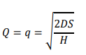
Where, S= setup cost per order, and H= holding cost per unit.

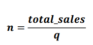
• Cycle Time (t) and Number of Inventory Runs (n):

a) Cycle time (t) was calculated as: 
b) The number of inventory runs (n) was calculated by dividing total demand by the order quantity.

Inventory Cost Analysis

The total expected inventory cost was computed by summing the setup cost, holding cost, and cost of stockouts.

Total Cost = Ordering Cost + Holding Cost + Stockout Cost

Definitions

• Inventory model: An inventory model is a mathematical tool used to determine the optimal order quantity, reorder points, and inventory levels to minimize costs while ensuring products are available to meet demand.

• Economic Order Quantity (EOQ): The optimal order quantity that minimizes total inventory costs.

• Reorder Point (ROP): The inventory level at which new stock should be ordered to avoid running out of the item.

Discussions

Analysis of Queuing and Inventory Metrics

a) Sales Performance: The business recorded a total of 23,042 transactions, generating an impressive sales revenue of $6,012,139. On average, each transaction involved the purchase of 1.24 items, with an average transaction amount of $260.92. Transaction values varied widely, ranging from $0 (likely due to returns or adjustments) to a maximum of $3,566.44.

b) Transaction Timing: On average, there was a gap of approximately 5.2 minutes (311.95 seconds) between transactions, which reflects both service efficiency and customer demand. The first recorded transaction occurred on August 1, 2024, at 12:43 PM, while the last transaction was completed on October 23, 2024, at 4:03 PM. Over this period, the total active sales time spanned about 83 days, indicating continuous business activity. Interestingly, the average service time per transaction aligns with the inter- transaction interval, suggesting a steady pace of operations. These insights highlight consistent operational performance, steady customer flow, and effective inventory movement, all critical for driving business success.

c) Insights

• Average Daily Demand: The average sales per day for each item are calculated. For example, Butter Naan has a high average daily demand of 23.3 units.

• Adjusted Demand: A 10% waste factor has been applied to the average daily demand, increasing the required stock for each item to account for possible wastage or overstocking.

• Reorder Point: The reorder point is calculated as Adjusted Demand * Lead Time (2 days) to ensure that inventory levels are replenished before stock runs out. Economic Order Quantity (EOQ): This helps determine the optimal order quantity for minimizing both ordering and holding costs. For example, Butter Naan requires an order quantity of 612 units.

• Total Cost: This includes the purchase cost, ordering cost, and holding cost for each food item. Butter Naan has the highest total cost due to its high demand and EOQ.

Inventory Model:

                                                                       Table 3: Sum of Revenue Get from Dine-In and Pick Up

A total of 170 items were sold across both channels, generating 55,335 rupees in revenue. The majority of the sales came from Dine-In, with 114 items sold, contributing 37,107 rupees (67% of total revenue). The remaining 56 items were sold through Pick-Up, generating 18,228 rupees (33% of total revenue).

                                                                 Table 4: Customers’ Payment Types in Restaurants

UPI (Other) is the dominant payment method, accounting for more than half of all sales revenue and nearly 60% of the items sold. Card Payments also play a significant role in sales, representing a third of the revenue. Cash and Part Payment are less commonly used, contributing relatively little to the overall sales.

                                                               Table 5: Quantity of Items at Tables in Restaurant’s Data

Row 1Label 3 and Row 1Label 16 have the highest sales, each contributing 15. The Row 1Label highlights the distribution of quantities across various Row 1labels, including numerical values, an alphanumeric label ("A"), and a "(blank)" category. The "(blank)" category stands out, contributing the largest share (56.00, 32.94% of the total). Significant contributors include Row 1labels "3" and "16" (each 15.00) and Row 1Label 2 (14.00), while Row 1Labels "1", "6", 9", "10", and "11" contribute minimally (each ≤ 3.00). The total quantity across all labels is 170.00. To improve the dataset's quality, it is recommended to investigate the "(blank)" category, prioritize high- contributing Row 1labels, evaluate the relevance of low-contributing ones, and ensure consistent data entry. Addressing these issues will enhance the dataset's reliability and analytical value.

                                                        Table 6: Quantity of Items at Tables in Restaurant’s Data

The time interval is 11-16 and 19-23. The total time 11 hours. This Table 6 summarizes the distribution of quantities across Row labels, totaling 170.00. High-contributing Row labels like 21 (39.00), 20 (29.00), and 14 (26.00) dominate the dataset, while mid-range Row labels such as 19 and 22 (each 16.00) and low contributors like 11 and 23 (each ≤ 2.00 ) add varying levels of detail. Addressing data inconsistencies and focusing on the high contributors can improve analysis and insights.

Transaction Timing Analysis

The time between transactions (Inter-Transaction Time) was, on average, 311.95 seconds. Large deviations in this metric suggest that the store’s customer flow could be more consistent with improved staffing and customer management. Transactions during off-peak hours (early morning or late evening) should be analysed further to determine if there are missed sales opportunities.

Sales and Inventory Optimization

The average quantity sold per item is relatively low, suggesting that bulk purchases or multi- item promotions could encourage higher sales volumes for certain products. Peak hours and days should be leveraged for stock replenishment. For example, sales on Sundays are particularly high, and focusing on stock management during weekends is crucial.

Service Efficiency

Service time and transaction time showed considerable variation. Long service times could be reduced by introducing technologies such as self-checkouts or increasing staff during peak hours. Investigating transaction times can provide insights into how staff efficiency or customer service may affect overall sales.

Summary and Conclusions

The objective of this Case study was to highlight the importance of understanding demand patterns and calculating the appropriate reorder points and EOQ for effective inventory management. For high-demand items, it is crucial to maintain adequate stock levels to avoid stockouts and maximize sales potential. The total cost of ordering and holding inventory should be carefully managed to ensure profitability. The business can use these insights to improve its procurement and stock management strategies, reduce waste, and enhance overall operational efficiency. inventory management systems of a business through a hybrid model approach, which included data collection, cleaning, and analysis to assess key performance indicators. This investigation yielded several significant insights regarding the efficiency of the service system and inventory management practices [1-14].

The principal findings are as follows

• Average Daily Demand Analysis: The study calculated the average daily demand for all 259 menu items. This provides a clear understanding of the consumption pattern of each item.

• Waste Factor Inclusion: A 10% waste factor was applied to the demand estimates to account for variability and potential spoilage. This ensures adequate stock levels while minimizing the risk of wastage.

• Reorder Point Calculation: The reorder point for each item was determined based on a lead time of 2 days. This ensures timely replenishment, preventing stockouts during peak demand periods.

• Economic Order Quantity (EOQ): EOQ was calculated for all items to identify the optimal order size, balancing the trade-off between ordering costs and holding costs.

• Annual Demand Estimation: By extrapolating daily adjusted demand to an annual scale, the analysis highlighted items with the highest consumption, such as Butter Naan and Chicken Dum Biryani, which require priority in inventory planning.

• Cost Analysis: Total costs, including purchasing, holding, and ordering costs, were calculated for each item. Items with high costs were identified, providing opportunities for focused cost-reduction strategies.

• Item Prioritization: High-demand items (e.g., Butter Naan with an annual demand of 9364 units) and low-demand items (e.g., Avakaya Chicken Biryani with 402 units annually) were identified, aiding in prioritization for procurement and inventory storage.

Recommendations to the Business Owner

• Stock Management: Focus on items with high demand, such as Butter Naan, which would benefit from frequent restocking and efficient inventory management to reduce holding costs.

• Ordering Frequency: Items like Butter Naan and Chicken Dum Biryani have large EOQs, indicating that they should be ordered in bulk at longer intervals to minimize ordering costs.

• Waste Reduction: The waste factor could be adjusted based on actual sales data. For some items, the waste factor may be higher or lower depending on the consistency of demand.

• Optimization of Costs: Reevaluate the ordering and holding costs periodically to ensure that the EOQ remains optimal as costs fluctuate.

• Focus on High-Demand Items: Items such as Butter Naan, Apricot Delight, and Chicken Dum Biryani, which have higher average daily demands and total costs, should be prioritized for better demand forecasting and stock management. Between 8 PM and 11 PM to maximize peak transaction periods.

Acknowledgements

I am grateful for the insightful comments offered by the anonymous peer reviewers.

Author Contributions

Sarode Shirisha Paper Writing, Abhirami KR and Akshay Krishnan Data collection and Methodology, Prof. Tirupathi Rao Padi Designed Paper. All authors critically reviewed and approved the final version of the manuscript for submission.

References

1. Sinuany-Stern, Z., & Sherman, H. D. (2014). Operations research in the public sector and nonprofit organizations. Annals of Operations Research, 221(1), 1-8.
2. Zipkin, P. H. (2000). Foundations of inventory management. McGraw-Hill. Irwin, New York, USA.
3. Skouri, K., & Papachristos, S. (2002). A continuous review inventory model, with deteriorating items, time-varying demand, linear replenishment cost, partially time-varying backlogging. Applied Mathematical Modelling, 26(5), 603-617.
4. Sicilia, J., San-José, L. A., & García-Laguna, J. (2009). An optimal replenishment policy for an EOQ model with partial backlogging. Annals of Operations Research, 169(1), 93-115.
5. Blos, M. F., Quaddus, M., Wee, H. M., & Watanabe, K. (2009). Supply chain risk management (SCRM): a case study on the automotive and electronic industries in Brazil. Supply Chain Management: An International Journal, 14(4), 247-252.
6. Sardroud, J. M. (2012). Influence of RFID technology on automated management of construction materials and components. Scientia Iranica, 19(3), 381-392.
7. Silver, E. A., Pyke, D. F., & Thomas, D. J. (2016). Inventory and production management in supply chains. CRC press.
8. Sampson, S. E., & Spring, M. (2012). Customer roles in service supply chains and opportunities for innovation. Journal of Supply Chain Management, 48(4), 30-50.
9. Fithri, P., Hasan, A., & Asri, F. M. (2019). Analysis of inventory control by using economic order quantity model–A case study in PT semen padang. Jurnal Optimasi Sistem Industri, 18(2), 116-124.
10. Farmaciawaty, D. A., Basri, M. H., Adiutama, A., Widjaja, F. B., & Rachmania, I. N. (2020). Inventory level improvement in pharmacy company using probabilistic EOQ model and two echelon inventory: a case study. The Asian Journal of Technology Management, 13(3), 229-242.
11. Geoffrey, K. K., Kaitany, P., & Sang, H. (2021). Economic order quantity stock control technique and performance of selected level five hospitals: An evidence of Kenya. International journal of business marketing and management, 6(6), 08-13.
12. Inventory Management Basics: Khan Academy
13. APICS (Association for Supply Chain Management): Offers guides on best practices in inventory and supply chain management.
14. Mohagheghi, O., Rezvani, S., & Hassannayebi, E. (2025, September). Stochastic optimization approaches to biomass- to-bioenergy supply chain network design under demand uncertainty. In Operations Research Forum (Vol. 6, No. 3, pp. 1-25). Springer International Publishing.