Exponential Function as a Polynomial of Non-Integer and Negative Exponents Newton Binomial Theorem Generalization Fractional Derivative of a Constant

Introduction

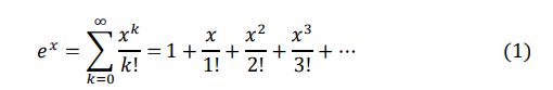
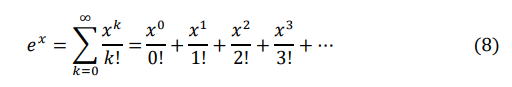
The exponential function is normally defined as the following power series [1]. In this definition the powers are positive integers:

In this paper, we will look for different power series but with non-integer (and also negative) exponents.

To do so, we will apply two methods.

The first one, more formal, will take use of fractional derivative. Normally the derivative is defined using integer ordinals, first derivative, second derivative etc.… The fractional derivative permits making such things as half derivative, 3/2 derivative etc.… We will use the non-written rule that whatever derivative we apply to the exponential function, the result should be the exponential function again. This way we will calculate the coefficients of the different power series [2].

The second one, much easier, will just make a generalization of the factorials that apply in the coefficient of the standard series (using the Euler gamma function [3]). And then using certain properties of this gamma function, we will operate them to try to obtain results that converge.

As a parallel consequence, these calculations will lead to a specific definition of the fractional derivative of a constant. It will be shown that there are multiple possible definitions for fractional derivative of a constant. But there is only one that at the same time fulfills the non-written rule that whatever derivative we apply to the exponential function we obtain again the exponential function.

Finally, a proposal for steps to go to a deeper generalization of the Newton generalized binomial theorem will be commented. Getting series of the Newton binomial composed by powers with non-integer exponents could be used in the Riemann zeta function, to find new ways of operating with it. Regretfully, this work has still to be done, as no valid solution has been found at this stage.

Applying the Half Derivative to the Exponential Function

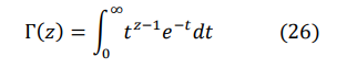
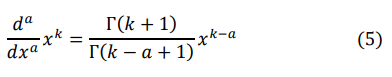
The fractional derivative of a power is defined as [2].

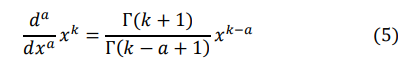
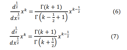
Where Γ represents the Euler gamma function [3]. So, to calculate the half derivative we substitute the “a” variable by ½:

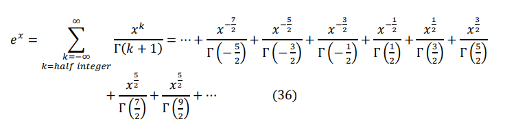
As commented before, the exponential function is defined as [1].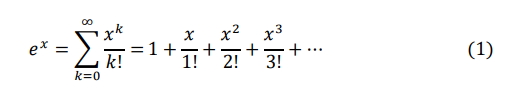

Our idea is to take the half derivative of the exponential function, taking the half derivative of each component. But, first, let’s make some cosmetic changes to facilitate this operation.

First, we will express the constant “1” as a function of x (in fact, as x^₀). And we will apply for this element also, the correspondent “hidden” factorial 0!. For the second element, we will make explicit the exponent 1.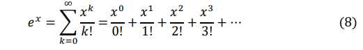

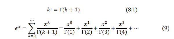
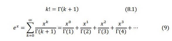
Now, we will substitute the factorials by its correspondent value of the Euler gamma func-tion knowing that [3].

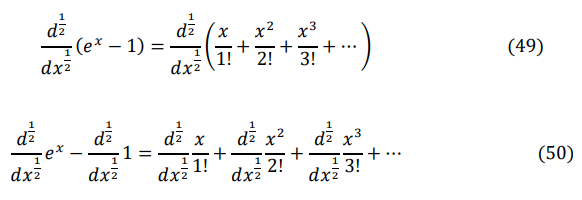
So, what we will do is to take the half derivative of each element, using the previous com-mented equation (7):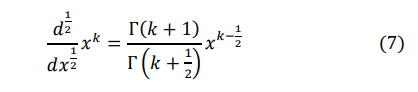

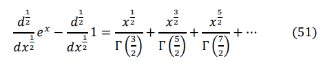
So, applying (7), element to element to equation (9) we obtain: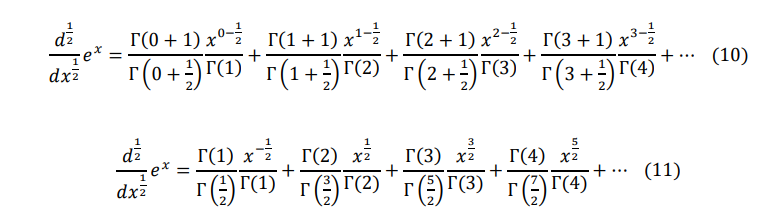

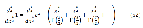
We can see that some gammas cancel each other (they are in numerators and denomina-tors). So, operating: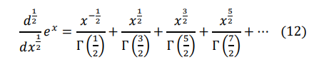

The problem with the expression (12) is that it is not correct. If we consider the non-written rule that every derivative (fractional or not) of the exponential function should be equal to the exponential function, this function (12) above does not fulfill it.

If you substitute the “x” above by different numbers, you will see that the result is not equal to ex. The higher the “x” you will see that they approximate but they are never the same. And with low values of “x” the distance can really increase. Check x=0, for example…

So, how do we correct it? We will oblige that expression to fulfil the rule that every deriv-ative we make, we get the same result (so forcing it to have the same property as the expo-nential function). So, how do we do it?

We do not need the fractional derivative anymore. We can just make the normal derivative once and again and check the results, until we get a result where the original is the same as its derivative (a property of the exponential function). So, we take the first derivative of  (12):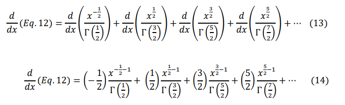 

Now, we will use the following property of the gamma function [3].

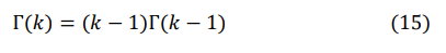
And I will apply it only to the elements that have exponents equal or higher than (-1/2) (later, you will see why):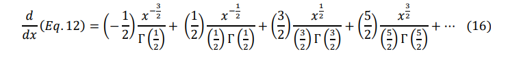

Cancelling the numbers that are in numerator and denominator, we have: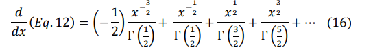

And you can check above that the equation (12) was: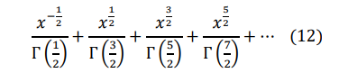

So, you can see that they are the same, except that a new element with exponent (-3/2) has appeared in (16). The rest of the elements (taking into account the … on the right) are the same.

So, we will take the derivative again (now to expression (16)) and see what happens: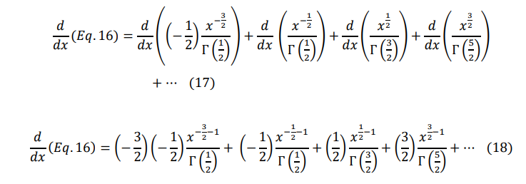

Making the substitution (15) for exponents equal or higher than (-1/2) we get: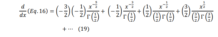

Leading to:

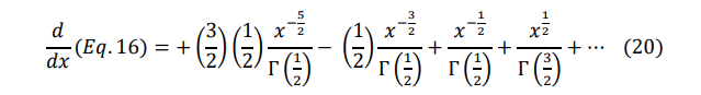
If we compare with expression (16), we see that they are the same but with a new element with exponent (-5/2). If repeat the process again and again (take the derivative again and again) we will get the expression: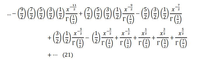

And if repeat the process infinite times, we get always the same result. We have infinite number of elements on the left and on the right, but if we take the derivative of all these infinite elements, we get the same expression. This means, the expression (21) fulfills the property that it is its own derivative (the property necessary to be a possible expression for the exponential function e^x).

But let’s continue cleaning a little bit the expression. For the elements with negative expo-nents, we will multiply the numerator and the denominator by Γ(1/2),leading to:

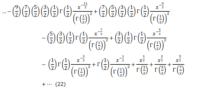
Now, using recursively the equation (15), we can check easily that for example:

so, applying this rule,where applicable, we get

 

 

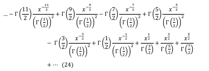
So, in principle this expression should be a candidate for the exponential function as a polynomial with non-integer exponents. It fulfills the property of being its own derivative. At least, it should be of the type k^.e^x (being k a constant, a scale factor). The problem is that the left side (the negative exponent side) does not converge. The gamma function value is increasing as we go to the left and it is in the numerator. You cannot just create a program to calculate one thousand elements and see the result (it will not converge). But this time,we have an escape. And surprisingly, it is based on the definition itself of the Euler gamma function [3]. 

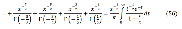
We will apply this definition to the elements with negative exponents and see what hap-pens: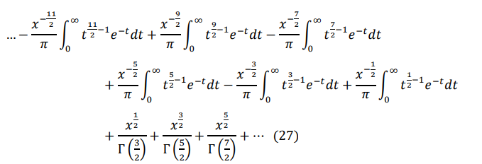

 

 

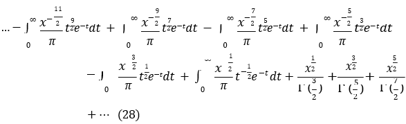
And as the integrals has the same limits and are a sum of integrals, we can take the integral of the sum of the integrands:

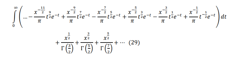
If we check the integrand form right to left, we can see that it is a geometric sum which first element is [4]. 

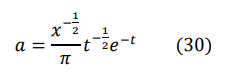
And the ratio is:

This geometric sum has infinite elements, so in theory, we need that the module of the ratio to be lower than 1, for the sum to converge. If we check the integral, the value of t goes from zero o infinity, so this restriction is not fulfilled. But the elements are multiplied by e-t that tends to zero quicker than the increase of t, so finally we will see that the integral converges (we will check that later numerically).

The result of a geometric sum when there are infinite elements is the following (32) (if you consider that the following equation is only true when the last element tends to zero, let’s have a discussion about it in Annex A1):

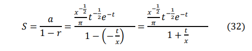
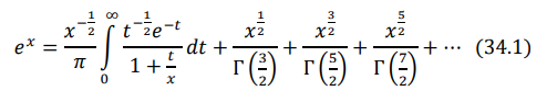
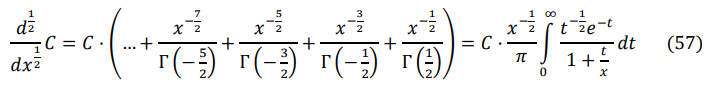
So, applying it to the equation (29) we get:

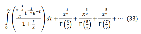
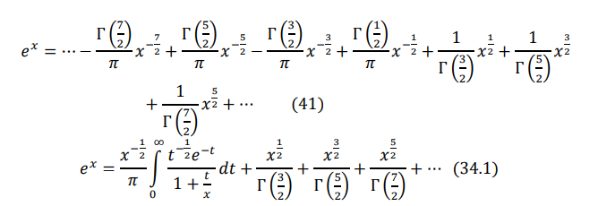
As x is an independent variable with respect to the integral, we can take it out: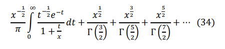

So, we get:

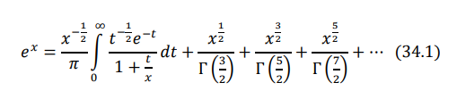
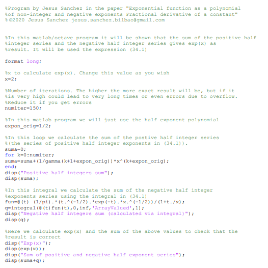
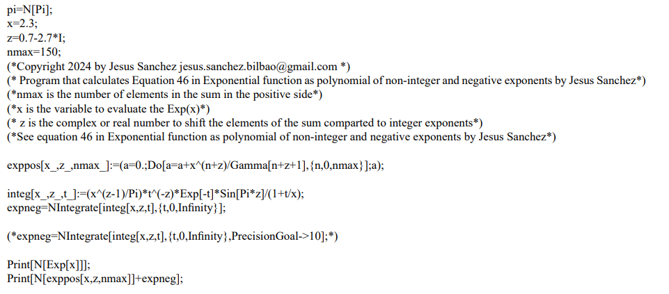
This integral can be calculated numerically. You can use online pages as or you can use the Matlab-Octave program included in Annex 1A to perform the calculation [5].

You can check that with the program in Annex A1, for x=2 we get:

Positive half integers sum

  7.052852096484307

Negative half integers sum (calculated via integral)

 0.336204002446341

Exp(x)

 7.389056098930650

Sum of positive and negative half exponent series

  7.389056098930649

And for x=3 we get:

Positive half integers sum

 19.798195673654210

Negative half integers sum (calculated via integral)

 0.287341249533456

Exp(x)

 20.085536923187668

Sum of positive and negative half exponent series

 20.085536923187664

As you can see, I have performed the calculation of ex using the expression (34.1) for different values of x, getting the correct result for ex. So, confirming that expression (34.1) is correct.

Getting the Same Result Using the Eulers Reflection Formula

Now, I will use another method to get to the same result. It is much easier and straightforward. But I wanted to show the previous one, as it is the one that uses the property that defines the exponential function (being its own derivative). Another reason I want to show this new method is because it will give us hints of how to apply it to generalize even more the Newton generalized binomial theorem [6].

This method is pretty straightforward. First, we have the definition of e^x [1].

We use equation (8.1) to arrive to equation (9):

Now, we generalize that equation for all the elements on the left (this means, the negative exponent elements that are hidden there):

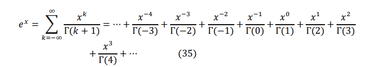
But, is this expression correct? Surprisingly again, the answer is yes. The gamma function for negative integers (and for zero) has infinite value. So, all the elements with negative exponents are zero. So, the expression (35) is equal to expression (9). The typical doubt here is what happens when x=0. This means we have zero multiplying infinity in the de-nominator. The answer is that the gamma function (or the factorial) always increases or decreases faster than a polynomial. So, the factorial always wins. In this case the infinity in the denominator of the factorial is “stronger” than the zero of the power, giving zero as result for each corresponding element.

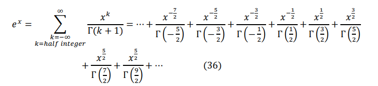
So why have we done this? Because of the next step. Now instead of integers, let’s put half integers for example (later we will generalize even more). We just exchange the integers by half integers, keeping the distance between them in one. And the corresponding gamma for each element, keeps being the exponent+1.

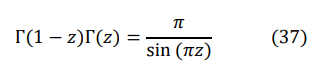
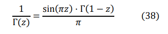
Now, we will use the Euler reflection formula for the elements that have negative expo-nents.

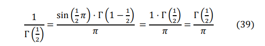
For example, let’s calculate for z=1/2.

Now, for z=-1/2:

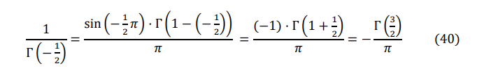
The last one, z=-3/2:

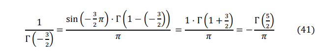
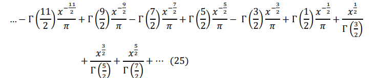
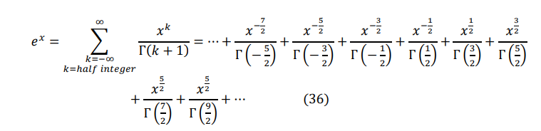
So, we can see the pattern. Let’s substitute in (36):

 

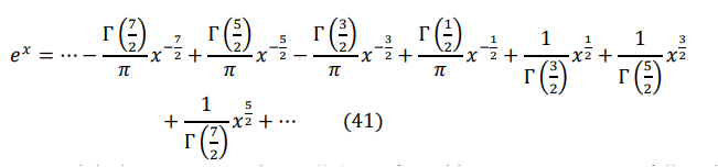
That we see, it is the same expression as (25). So, from this moment on, we can follow the same steps as in previous point (from equation (25) on), to arrive to the equation:

That we have seen in the previous point, that it is correct (after checking numerically with different values for x).

The reason I wanted to show this method is because of the expression (36):

 

This expression is correct, as it has been demonstrated a posteriori, after performing dif-ferent operations to arrive to a correct result. But the importance of the equation (36) is that it has been obtained not applying any rule (like keeping the derivative or similar), just generalizing the expression (35) changing the numbers, and it has worked! This gives some hope, if something similar can be done with the binomial theorem to get to correct results being able to obtain polynomials of non- integer exponents.

Another thing we can see with this expression (and also really with the fractional derivative we have seen in previous point) is that it is not necessary that k is half integer. k can be whatever number (even complex). And the only rule we have to follow is that the steps between one element and the next is 1. The difference between k in one element to the next should be one. But apart from that we can choose whatever k. For example:

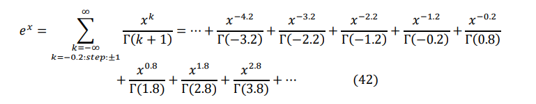
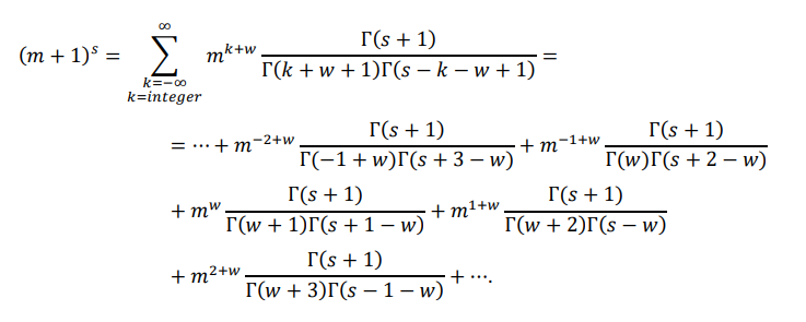
Is correct. So, in general, we can say something like (for whatever complex number z, being k integers):

 

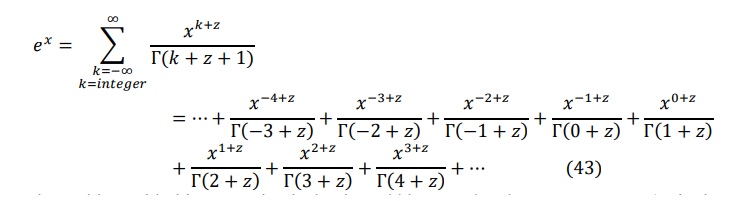
The problem with this expression is that it could happen that does not converge (or in the left side or in the right side). In that case, the Euler reflection formula (37) could be used to try to change the position (numerator, denominator) of the divergent elements. If this does not work, try using the definition of gamma looking for a convergent integral, as I have done in the first point. Another tool that is available (mainly when half integers are involved) is the double factorial division between odd and even double factorials when they are generalized as complex numbers. The last tool I can think of is the convolu-tion theorem in case that you arrive to a situation that you need to multiply two integrals corresponding to two gamma functions. I comment them here even if in the end I did not use them, but in case they could be useful. The division between double factorials could be key regarding the Riemann zeta function, as when the real part is ½ (really is -1/2 in the calculations), to get the division between double factorials is very common when you apply the binomial theorem to a component of the function [7,8].

We can also convert all the negative exponents in an integral as we made before, the fol-lowing way:

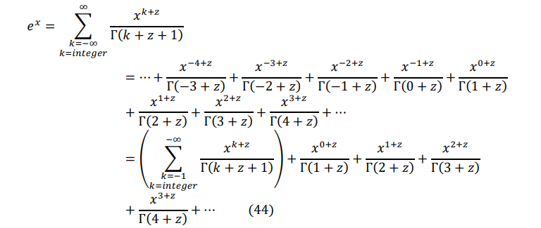
We will calculate only the part between brackets (later we will return here):

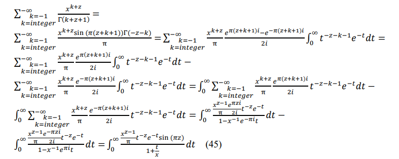
So, coming back to (44):

You can check that the equations (42) to (46) are correct using the Matlab or the Mathe-matica programs in Annexes A5 and A6 for the expresion (46) that is a generalization of all of them.

Also, the equations that have been proved to be true both analytically and numerically are the equations from (33) to (41) (including the 34.1). These are the ones that correspond to half integer exponents. These equations have been derived analytically and have been cal- culated numerically with a Matlab/Octave program -Annex A1- (and can be rechecked with online integral calculator resources as [5]). See examples in Chapter 2, after (34.1) equa-tion.

Fractional Derivative of a Constant

Now, that we have seen how to make the fractional derivative of the elements of the expo-nential function, we can use this information to calculate the fractional derivative of a con-stant. There is the debate if the fractional derivative of a constant is directly zero or if it is the result according following definition when k=0 [2].

This is:

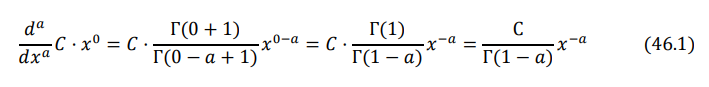
For example, when a=1/2

And, in fact, if you take the half derivative again of that expression, you will get 0 (as it is expected for having made two times the half derivative to a constant). The reason is that you will get a Γ(0), that is infinity, in the denominator. And this leads to a final result of zero to the expression.

The issue is that it is not the only valid solution. There are infinity of them, see for example:

If you take the half derivative, you will obtain a Γ(-1) in the denominator, that is also in-finity. Giving the result as zero. Even a combination of them such as:

Will lead to zero in the next half derivative (due to Γ(0) and Γ(-1) in the denominators) . So, there are infinite solutions for the half derivative of a constant. So which one shall we use? We will use again the exponential function to find the most appropriate one. Let’s use this expression:

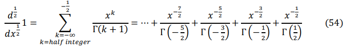
And now, let’s take the half derivative:

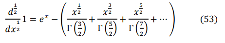
Now, calculating as in equations (10), (11) and (12) we get:

Now, if isolate the fractional derivative of 1 and change the signs of both sides we have:

On the other side, we have the non-written rule that whatever derivative of the exponential function is itself so:

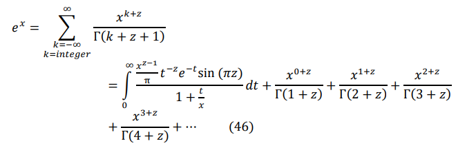
And, remember we had this definition for ex in equation (36):

If we substitute equation (36) in the ex of equation (52) and perform the subtraction we get:

For whatever constant C, it would be:

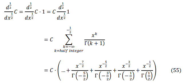
Also, as we have seen in equation (34), we know that:

So:

 

This expression is the only one that fulfills at the same time, that the next half derivative will be zero (as expected for a constant), but also that the fractional derivative of the exponential of x keeps being the exponential of x.

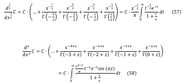
If we generalize for other fractional derivatives we would obtain (see 44 and 46):

 

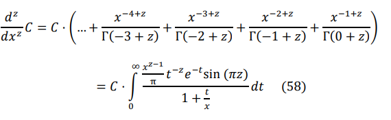
As commented in chapter 3 (after equation (46)), the equation (57) has been obtained analytically and demonstrated numerically. This is not the case for equation (58) that has to be rechecked numerically to be completely validated.

Generalization of the Newton Binomial

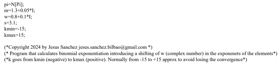
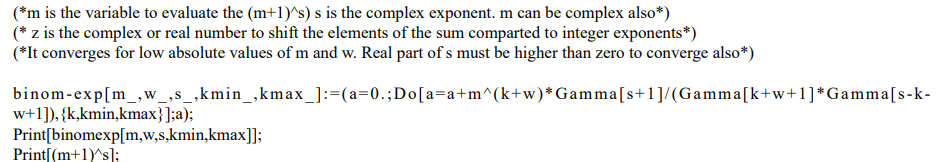
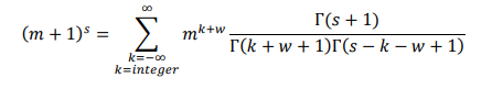
Another similar equation that can be used with the Newton binomial is the following:

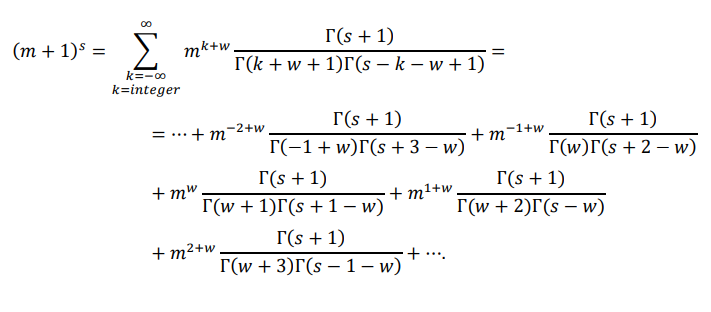
You can find in Annex 7 a Mathematica program that performs this calculation. All m, w and s can be complex numbers. But m and w have to be of low absolute values (in the order of 1 or less) to converge. Also, the real part of s has to be higher than zero. Also, the limits of k have to be controlled, giving from -15 to +15 the best results. As you can check, w is a free parameter that you can define as it best suits your necessities.

Clearly the use of this equation is not to perform the calculation (there are better ways).

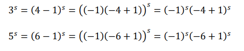
The use of this equation is to be used as a tool for other demonstrations. For example, it can be used in the Riemann zeta function to compute the odd numbers exponential as function of the even numbers this way:

And try to use it to manipulate somehow the elements. You can select w so some gamma functions or similar can be computed or cancelled. You can check all the properties of the gamma functions in [3]. You can play with them and try to obtain new properties of the gamma function for example.

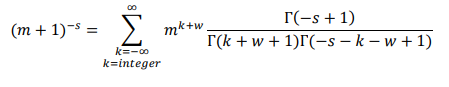
You can calculate also these other equations for example:

And to try to manipulate the different elements subtracting or summing to higher above equation for example. You can see an example of use of above equation to obtain the sum of Riemann zeta function series in Annex A8.

Conclusion

The main goal of the paper was to obtain a generalization of the series expansion of the exponential function with non-integer exponents polynomials. We have shown analytically and numerically that the following expansion are correct:

The Newton binomial theorem is also generalized this way (being w a free complex parameter):

Also, we have shown that the only definition of fractional derivative of a constant that at the same time keeps the rule that any differentiation of the exponential function has to be itself again is the following:

Also, in the annexes some considerations regarding the geometric series and some results for some of them are obtained (sin(nx) and cos(nx) series, sums related to Riemann Zeta Function etc….).

Gorliz, 18th August 2020 (viXra-v1).

Bilbao, 30th December 2023 (viXra-v2).

Bilbao, 31st December 2023 (viXra-v2.1)

Bilbao, 2nd January 2024 (viXra-v2.2)

Bilbao, 3rd February 2024 (viXra-v2.3)

Acknowledgments

To my family and friends, to Tea Brana, to Guillermo and Adso, to Pirataaaaaa, to Mikuo and Je, to Demi Akafe and to the unmoved mover.

References

1. https://en.wikipedia.org/wiki/Exponential_function
2. https://en.wikipedia.org/wiki/Fractional_calculus
3. https://en.wikipedia.org/wiki/Gamma_function
4. https://en.wikipedia.org/wiki/Geometric_series
5. https://www.integral-calculator.com/
6. https://en.wikipedia.org/wiki/Binomial_theorem#Newton's_generalized_binomial_theorem
7. https://en.wikipedia.org/wiki/Double_factorial
8. https://en.wikipedia.org/wiki/Convolution_theorem
9. https://mathworld.wolfram.com/RiemannZetaFunction.html
10. https://keisan.casio.com/exec/system/1180573439
11. https://en.wikipedia.org/wiki/Riemann_zeta_function
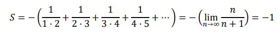
12. https://socratic.org/questions/598f653ab72cff3fe6b13051
13. https://www.quora.com/How-do-I-solve-1-2-+-1-6-+-1-12-+-1-20-+-1-30-+-1-42-+-1-56-+-1-72-+-1-90-+-1-110-+-1-132
14. https://en.wikipedia.org/wiki/Taylor_series

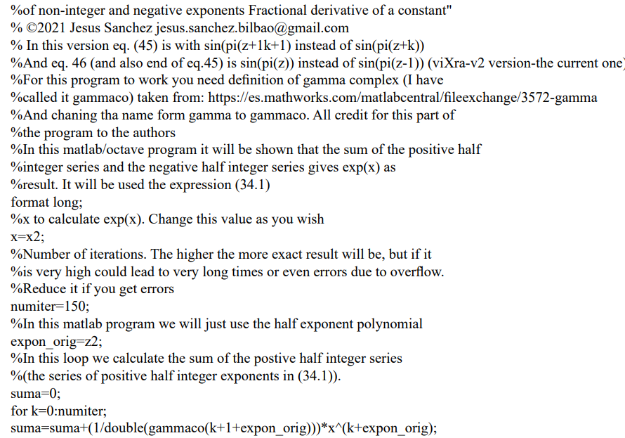
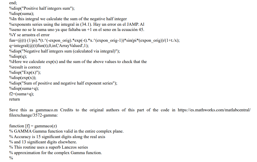
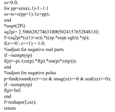
  A1. Annex A1. Matlab/Octave Program for Expression (34.1)

  You can find here attached a program in Matlab/Octave to calculate the expression (34.1) and check that the result is the same as     the exponential of (x)

A2. Annex A2. If a series does not no converge, it does not mean that the result of its sum is incorrect

Let’s calculate the sum of a geometric series. We will follow the rules and we will choose a series which last element tends to zero.

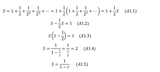
If we take a calculator and we start summing elements:

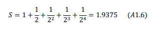
And we take more and more elements we see that we approach the final result S=2. But this is misleading, because the reality is that in the real world we will never get the result S=2. We will get there only if we are able to sum “all” the elements. And in that case, we will get the result S=2. If not, we will be nearer and nearer but never arriving. Ok, now let’s not follow the rules. Let’s try to get the sum of the following geometric sum. The last element does not tend to zero (the opposite, is increasing continuously):

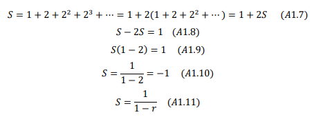
We have followed exactly the same steps as in (A1.1 to A1.5). So, this procedure is as correct or as wrong as before. There is nothing that tells us that we have to apply an “ad hoc” extra rule to this result. Both calculations are ok or both calculations are wrong.

So, what is the difference? In the first case (A1.1), if we are not able to calculate the result, we can use the “trick” of summing a lot of elements to check if they approach something. In the second case (A1.7) this trick does not work. But, in fact, this is the only difference between both cases.

Both cases have something in common. We are not able, as human beings, to perform the total sum of the elements. We will never sum all the elements in the first case (A1.1), and we will never sum all the elements in the second case (A1.7).

But everything points to, that if we were able to do it (to sum all the elements), we would get S=2 in the first case and S=-1 in the second case. But we are not able to do it (neither in the first case and neither in the second). Yes, if we were able to sum all the elements in the second case, we would get S=-1 (but we are not able to do it). Exactly the same that we would get S=2 in the first case (but we are not able to do it).

Both results are ok or both results are wrong. But it is not the case the first one is ok and the second not. Normally it is said that the second case (A1.7) is an artifact (an extension of a result that does not have any meaning). But it is really the opposite. The artifact is in our minds, that as we cannot understand that result, we impose the condition that it is not possible or incorrect. But there is nothing incorrect in the steps followed (at least as incor-rect as the first case (A1.1) can be). The artifact is in our minds, imposing an “ad hoc” rule just because we do not understand the result. But the numbers do not lie, if we were able to make the sum of “all” the elements in (A1.7) the result would be S=-1. But we are not able to sum all the elements, so we cannot check it. The numbers do not care if we are able to understand it or not, they just tell us that that is the result. The result for (A1.7) is as correct or as incorrect that (A1.1) is S=2 (that is something that really, we cannot check also, we are not able to make the complete sum).

The only difference between first case (A1.1) and second case (A1.7) is that in the first case, we can try to approach the result making partial sums. In the second case, we must sum all the elements to get the result. The trick of partial sums does not work. And as we are not able to make the total sum of all the elements, we consider that the result is incorrect. The artifact is not the result, the artifact is the conclusion that there must be something wrong here just because we are not able to perform that sum including all the elements.

A3. Annex A3. Offtopic. Sum of sin(nx) and cos(nx) series

Once we have internalized the Annex A2, we can start making sums which last element does not tend to zero and see that we get results.

For example, we can start with the sin(nx) series:

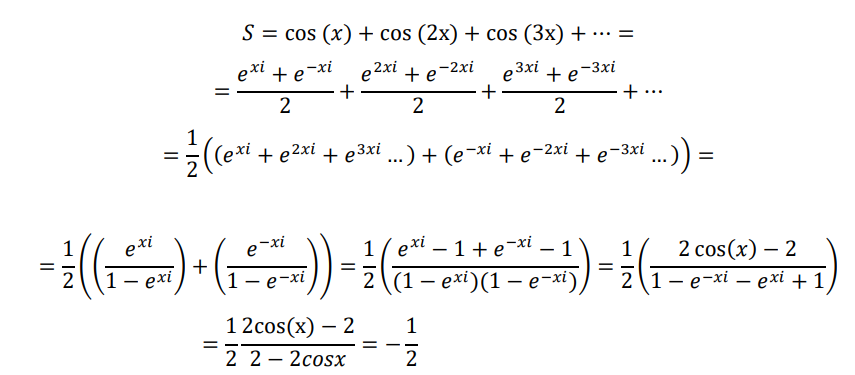
And we can get a result also with the cos(nx) series:

A4. Annex A4. Offtopic. Sum of Riemann zeta function series

Let’s calculate the following sum. This calculation is not original, you can find the result for example in [9]. But we will use it as an example of what it will come later (jump to A4.1 if you want):

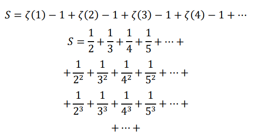
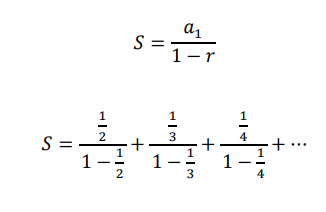
If we check the columns, we see that they are geometric sums, so we can use the geometric sum equation [4].

 

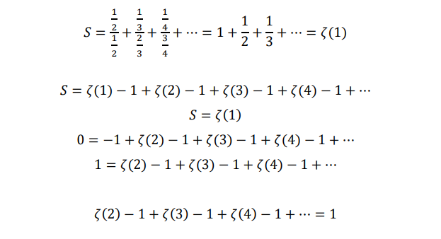
We can check that this is correct just operating numerically. You can find the values of the Riemann zeta function here [9-11].

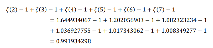
And the higher number of elements, we include the nearer we go to 1.

But what has not been ever commented is that we can make the same sum but for all the elements (not only the positive ones), getting the result zero.

 

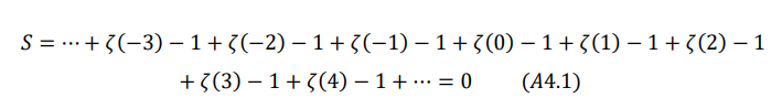
This sum can be performed even if the negative elements does not tend to zero. This is only possible if we take the Annex A1 into account.

To demonstrate this, let’s make a partial sum starting in ζ(-1):

 

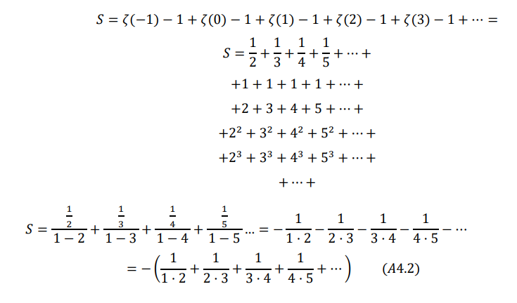
The sum in brackets is 1, as you can check in where a general sum of this type with n terms is calculated [12,13].

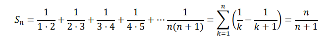
When we have an infinite number of elements n is infinite giving as result 1 when n tends to infinity, so coming back to (A4.2):

So, coming back to (A4.1):

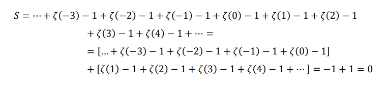
We can get this result cutting the sum wherever we want, so in general we can say that:

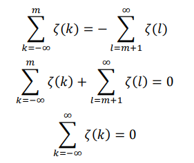
As commented, this would not have any meaning or we could not even think about it, if we do not consider that what is commented in Annex A1 is correct.

A5. Annex A5. Matlab/Octave Program for Expression (46)

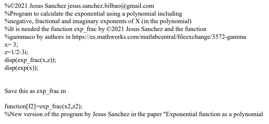
You can find here attached a program in Matlab/Octave to calculate the expression (46) and check that the result is the same as the exponential of (x).

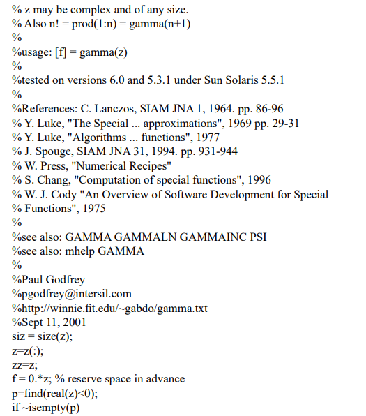
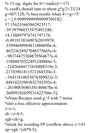
The functions afterwards should be saved in matlab with the names exp_frac.m and gammaco.m to work. Gammaco function comes from https://es.mathworks.com/matlabcentral/fileexchange/3572-gamma with its corresponding credit to the authors.

Save the following one as exp_frac_main.m

A6. Annex A6. Mathematica Program for Expression (46)

A7. Annex A7. Mathematica Program for Generalization of Binomial Theorem

 

A8. Sum of infinite Riemann Zeta Functions

In chapter 4 we obtained:

That can be modified as:

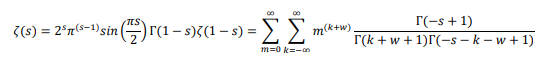
So, Riemann Zeta function can be expressed as:

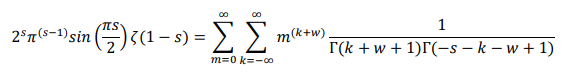
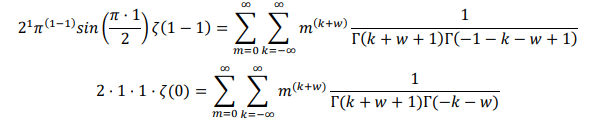
Being w whatever complex number we want to choose (it is a free parameter). Applying the functional equation to the Zeta Riemann function [9].

We can cancel the elements Γ (1 - s ) and Γ ( s - 1) in both sides of the equation as they are the same:

If we apply for s  = 1:

We can use the Euler’s reflection formula of the Gamma function [3].

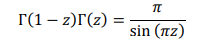
Considering z and 1-z as follows:

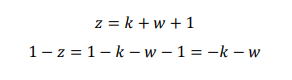
So:

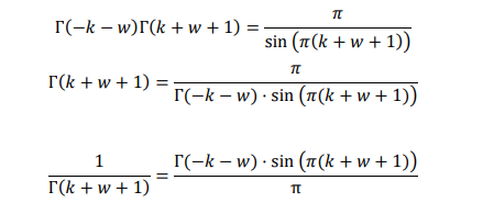
Applying it to the higher above previous equation

 

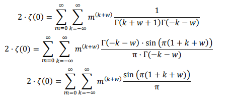
The factor of the sin is periodic. When k is odd, it is positive. And when k is even, it is negative, as you check. So:

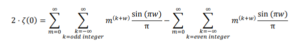
Now, we can make a change in the definition of k (not changing the real terms or the in-herent meaning of the distribution of terms), to represent above formula this way:

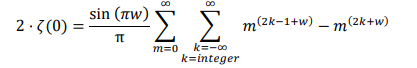
Exchanging the summations of m and k (as they are independent):

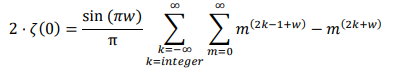
By definition of Riemann Zetafunction [9].

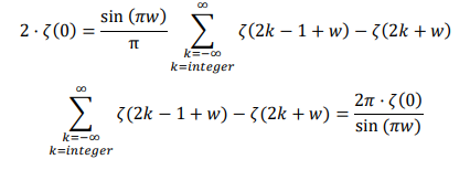
Riemann Zeta function for s=0 is equal to -1/2 [9].

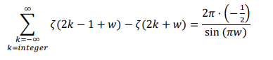
So, finally we get the following equation for whatever complex number w we want to choose (it is a free parameter):

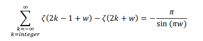
The representation with explicit terms would be

A9. Taylor series with non-integer exponents

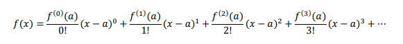
We know the classical expression of the Taylor series [14].

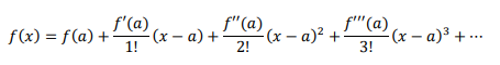
Using the superscript (n) for the function f, meaning the order of derivative, this can be represented as:

 

But as we have seen throughout this paper (chapters 2 on), we can generalize above expression using fractional calculus [2]. The fractional calculus permits to have fractional or even complex derivatives. In fractional calculus a negative superscript would mean fractional integral.

So, we can generalize the Taylor series as follows, following the same criteria used in this paper. This is, substituting factorials by Gamma function of the factorial+1 and making the sum for all the components from -infinity to + infinity (instead of only the positive ones, used in traditional polyno-mial series):

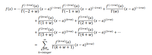
Being w whatever complex number we want to choose (it is a free parameter). And the superscript (k+w) in the f, meaning the order of the fractional derivative (or fractional integral if it is negative) applied to the function f.