
Journal of Applied Material Science & Engineering Research(AMSE)
ISSN: 2689-1204 | DOI: 10.33140/AMSE
Impact Factor: 0.98

Research Article - (2024) Volume 8, Issue 2
Exploration of Multi-Label Classification Techniques for Modelling of Specialty Arabica Coffee Flavour Notes
Received Date: Apr 16, 2024 / Accepted Date: May 14, 2024 / Published Date: May 24, 2024
Copyright: ©Â©2024 S. H. S. Ho. This is an open-access article distributed under the terms of the Creative Commons Attribution License, which permits unrestricted use, distribution, and reproduction in any medium, provided the original author and source are credited.
Citation: Ho, S. H. S. (2024). Exploration of Multi-Label Classification Techniques for Modelling of Specialty Arabica Coffee Flavour Notes. J App Mat Sci & Engg Res, 8(2), 01-13.
Abstract
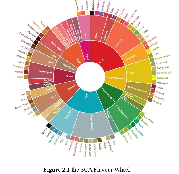
The world of specialty Arabica coffee transcends mere taste and aroma, offering a variety of distinct flavour notes that confer a unique sensory experience for each coffee. Capturing these unique flavours presents a major challenge, as descriptions of the same flavour notes by sensory evaluators can be extremely varied. The Specialty Coffee Association has come up with the Coffee Flavour Wheel in an attempt to align the tasting of coffee by providing a hierarchical framework of flavour descriptors [1].
Introduction
The world of specialty Arabica coffee transcends mere taste and aroma, offering a variety of distinct flavour notes that confer a unique sensory experience for each coffee. Capturing these unique flavours presents a major challenge, as descriptions of the same flavour notes by sensory evaluators can be extremely varied. The Specialty Coffee Association has come up with the Coffee Flavour Wheel in an attempt to align the tasting of coffee by providing a hierarchical framework of flavour descriptors [1].
Knowing and recording the flavour notes of Arabica coffee serves several purposes in the industry. One, it attempts to highlight the differences between coffee of various origins. Two, it guides companies in the coffee trade on the types of coffee to accept in pursuit of a consistent flavour profile. Three, it enhances the experience by consumers when choosing, purchasing and tasting different coffees. However, tasting flavour notes is not an easy task, and requires sensory panellists trained in the art of tasting coffee. Consequently, for any unknown coffee sample, it is necessary to assemble a group of trained panellists to taste and describe it, which could lead to mounting costs and long lead times.
In recent years, attempts have been made to solve this problem, generally by building supervised learning models to allow for inference of flavour notes in silico without the need for human panellist. Since coffee flavours have a basis in its chemical constituents, present methodologies typically employ a chemical analytical process on coffee beans, then finding an appropriate mapping to one or more flavour notes, whether directly or indirectly through quantitation of one or more specific compounds such as pyrazines or esters.
Caporaso et al. applied hyperspectral imaging in the near- infrared range on single roasted coffee beans to model the amounts of specific compounds such as aldehydes and pyrazines as determined by gas chromatography-mass spectrometry [2]. Esteban-Díez et al. employed near-infrared spectroscopy to build regression models to infer acidity, mouthfeel, bitterness and aftertaste in roasted coffee successfully but these inferred parameters are not as specific as those described by the flavour wheel [3]. Chang et al. similarly used near-infrared spectroscopy, albeit on roasted and ground coffee [4]. Modelling was done with an assortment of machine and deep learning techniques including support vector machines (SVM) and convolutional neural networks (CNN) to achieve accuracies in the 75-77% range in inferring the flavour notes corresponding to the innermost wheel of the SCA flavour wheel (Floral, Fruity, Sour/Fermented, Green/Vegetable, Other, Roasted, Spices, Nutty/Cocoa, Sweet). In the above three works, there is a clear progression. Firstly, near-infrared analysis of coffee was related to a more direct analysis through gas chromatography, but the relationship to an actual sensory description is not elucidated. Next, similar near-infrared was then used to relate directly to general sensory descriptions such as “acidity” and “mouthfeel” in a scored manner. Lastly, we see the most direct mapping from near-infrared to specific descriptors in the SCA flavour wheel in Chang et al.'s work.
There are a couple of salient points regarding the present state of the art. Many of the attempts to relate coffee to flavour have been done on roasted coffee beans or their resulting grounds, but there is merit as well in being able to infer a coffee bean’s flavour notes when it has not yet been roasted. On the modelling front, much work has involved building discrete models that each map certain features in the collected spectra to a specific flavour parameter, thereby necessitating multiple independent models to describe the flavour profile of a coffee. We discuss this in more detail.
Since a coffee sample could present multiple flavour notes according to the SCA flavour wheel, for example, having sour/ fermented, fruity, roasted flavours at once, this indicates that usual binary or multiclass classification is insufficient as these methods only infer one output result. In this case, multilabel classification is required in order to infer one or more labels for any sample. There are a few approaches to multilabel classification. At its simplest, an decomposed approach may be used, wherein several different multiclass classifiers are trained and used to infer an output each, which is then presented as a set of labels (multi-labels) for a data point. This is the approach used by Chang et al. above. Binary relevance, wherein for each label, a binary classifier is trained, and where the type of classifier for each label is the same, is typically considered to be the baseline multilabel approach [5]. An extension of the binary relevance method is classifier chains, wherein the binary classifiers are ‘chained’ such that succeeding classifiers incorporate the output from preceding classifiers as part of their input. The advantage of classifier chains is that they consider the possible correlations that may exist between the labels themselves.
In this present work, we examine the use of multilabel classification techniques to model flavour notes present in green unroasted coffee beans using visible near-infrared spectra of these beans as the input data. We consider a sequential exploration of techniques, starting with binary relevance, followed by an exploration of several classifier chain approaches and ending off with decomposed approaches. The development of a multilabel classification approach using unroasted coffee bean spectra is expected to facilitate the evaluation of coffee beans upstream in the supply chain without the need for cumbersome sensory evaluations.
Materials and Methods
Visible-Near-infrared Analysis of Green Coffee Beans and Labelling of Relevant Sensory Data
60 different lots of green, unroasted coffee beans were purchased from Sweet Maria’s (https://www.sweetmarias.com/), a coffee roaster headquartered in Oakland, CA, United States. For each sample, Sweet Maria provides a scoring of 0-5 for each of “Floral”, “Honey”, “Sugars”, “Caramel”, “Fruits”, “Citrus”,“Berry”, “Cocoa”, “Nuts”, “Rustic”, “Spice”, “Body” flavour notes. With the exception of “Rustic” and “Body”, the other ten flavour notes are represented either in the inner circle (“Floral”, “Fruits”, “Spice”) or the middle and outer circles (“Honey”, “Sugars”, “Berry”, “Citrus”, “Cocoa”, “Nuts”). These notes are labelled unto the respective beans as “present”, denoted by “1”, if the score is 1-5 or “absent”, denoted by “0” if the score is 0.
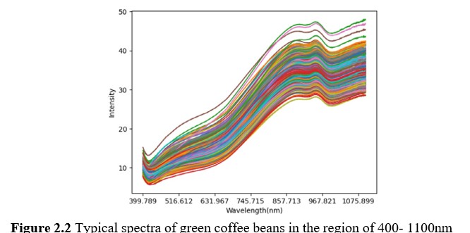
Scanning of coffee beans was done with the ProfilePrint analyser v3.0 (ProfilePrint Pte Ltd, Singapore), which illuminates the sample using a tungsten halogen light source and collects visible- near-infrared signals (400-1100nm) through diffuse reflection. 7 specimens of 8-10g each were drawn from each sample lot of coffee beans, resulting in 7 spectra for each lot.
â??â??â??â??â??â??â??Preprocessing of Spectral Data
Spectral data was collected in 0.3nm intervals, for a total of 1226 datapoints per spectrum. Each spectrum was then normalised through the Standard Normal Variate method in order to correct for surface irregularities as the scanned material were intact green coffee beans. Through this method, baseline and multiplicative effects are mitigated, allowing for better comparison between spectra [6]. Briefly, each spectrum is subtracted by its own mean and divided by its own standard deviation, thereby normalising all spectra to a mean of 0 and a standard deviation of 1.
â??â??â??â??â??â??â??Data Analysis and Modelling
All data analysis and modelling methods were implemented on a Python 3.0 platform through the Scikit-learn library [7]. Data analysis of the coffee spectral data was conducted using principal component analysis (PCA). PCA seeks to transform a high- dimensional data matrix into a lower-dimensional space while preserving the maximum amount of variance within the data. It achieves this by identifying a set of orthogonal uncorrelated vectors, known as principal components (PCs), that capture the directions of greatest variance in the data. In consideration that the data structure may not be linear in nature, kernel PCA (KPCA) was also employed. KPCA implicitly projects the data into a high-dimensional feature space through a nonlinear kernel function, enabling it to capture higher-order dependencies and nonlinearities not readily apparent in the original space. Subsequently, it performs PCA within this transformed space, effectively learning nonlinear principal components. In this work, the radial basis function (rbf) kernel was explored. Uniform Manifold Approximation and Projection (UMAP) has increased in popularity as an algorithm for dimensionality reduction and visualization in cell biology, particularly when applied to high-dimensional cellular data [8]. UMAP excels in unveiling local structures within the data while also preserving the global context. In the context of the discussed coffee spectra data, our employment of UMAP aimed to uncover insights at the local level, offering a nuanced perspective compared to PCA, which primarily emphasizes directions of variance of the whole dataset.
Classification modelling was performed with logistic regression, support vector machines (SVM), random forest (RF) and AdaBoost. Logistic regression employs a sigmoid function to map linear combinations of input features to the probability of a sample belonging to a class. SVM uses a variety of kernels (linear, polynomial, rbf) to project the data to higher dimensional spaces for separation by means of a hyperplane [9]. In this work, we explored only the versatile rbf kernel. RF and AdaBoost are tree-based classification methods. Whereas the former generates a ‘forest’ of decision trees which vote to conclude the class of a sample, the latter iteratively builds, or boosts, decision trees by focusing on the misclassifications of the preceding trees [10].
The above four classification algorithms formed the backbone of the multilabel classification techniques explored herein. Binary relevance was attempted, and this optimises the choice of algorithm and trains a model for all labels simultaneously, choosing the best algorithm for all attributes by minimising the Hamming loss [11]. Next, the classifier chain approach was attempted, whereby flavour notes thought to be related are chained such that the prediction output of the prior flavour note is an input feature for the subsequent flavor note(s). In other words, dependencies between labels are considered here [12]. A few variations were attempted. The first was to chain all binary flavour models together in a random arrangement. The second variation was to chain in a predetermined order as indicated by the results from the binary relevance experiment. The last variation was to create sub-chains where related flavours were chained together, presumably this would improve accuracy as correlated flavour notes would input into one another.
The Hamming loss is defined as:
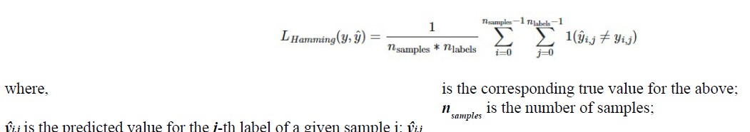
nlabels is the number of labels.
The dataset was split 80:20 into train and test sets. For the train set, a 5-fold cross validation (CV) was also conducted, and the choice of models was based on the model pipeline which generated the lowest cross validation Hamming loss. Subsequently, the model was tested on the test set and the test Hamming loss was calculated as well. Balanced accuracy was also calculated for the test set for each label, together with a mean balanced accuracy for all labels.â??â??â??â??â??â??â??
Results
Exploratory Data Analysis
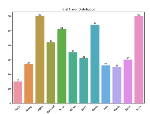
Figure 3.1 Flavour notes representation of coffee samples. Note that each coffee sample may be represented by one or more flavour notes.
The flavour notes representation of the 60 lots of green coffee are shown in Figure 3.1. There are a total of 12 flavour notes, but only nine flavour notes were shortlisted for further analysis and modelling. The three flavour notes omitted were “Rustic”, which is a flavour note not found on the SCA flavour wheel; and “Sugars” and “Body”, both of which were present in all 60 lots, and therefore unable to be modelled due to the lack of negative samples. Beyond that, several flavour notes were not represented in a balanced manner - “Floral”, “Fruits”, “Cocoa”. It would be insightful to look at how the modelling results would be for these notes.
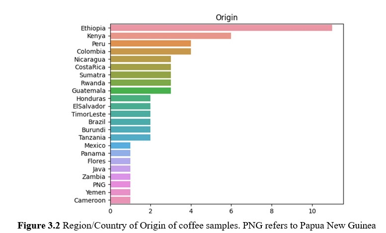
The coffee lots had a global representation, albeit with a relatively larger number of Ethiopian samples. It is noting that Indonesia is not represented as one country, but as three regions - Sumatra, Flores and Java, with the recognition that coffee beans from different regions of Indonesia differ significantly from one another. There are a total of five samples of Indonesian origin.
Principal Component Analysis
Principal component analysis was performed on the spectra of all 60 lots post preprocessing, with each lot presenting 7 data points as a result of 7 specimen samplings. The intention here is to investigate if the data showed any prominent directions of variance or clusters. According to Figure 3.3., it was however clear that the data distribution showed no clearly separated clusters even at deeper principal components. This suggested that as a whole, the distribution of the data was continuous with no attributable clusters to flavour notes nor origins. A closer look at the plot of PC1 versus PC2 does show a slight bias of samples with floral notes towards higher PC1 values and those without floral notes with lower PC1 values. The above observations similarly apply when the data points were coloured according to the presence or absence of the other eight flavour notes.
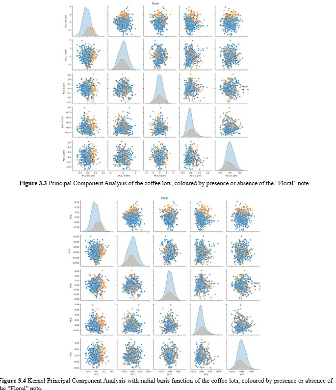
Next, kernel PCA was attempted with the data using the radial basis function (rbf), polynomial or cosine kernels in order to investigate for any significant presence of non-linear patterns in the data. Figure 3.4. depicts the PC plots as generated by processing the data through kernel PCA with the rbf kernel. Immediately obvious is the observation that the datapoints are almost exactly placed with the same relation to one another; only the numerical values of the principal components are different. This suggests that although the kernel has induced a transformation of datapoints into a distinct space compared to PCA without the kernel, the relationships between datapoints remain largely unchanged. This observation strongly implies that linear patterns dominate the data, and preprocessing may have effectively mitigated non-linear patterns. Notably, it is essentia to acknowledge that both polynomial and cosine kernels yielded similar projections of the data.
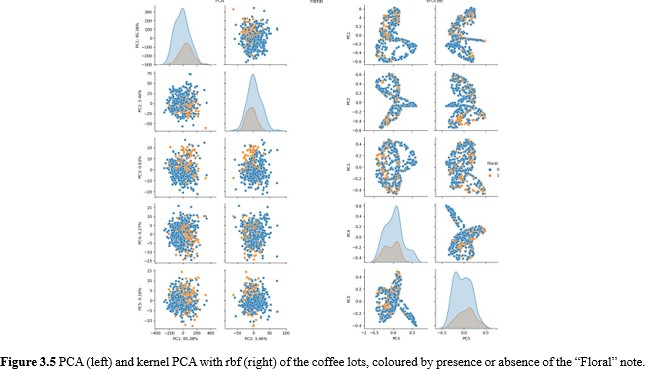
To investigate the above further, PCA and kernel PCA with the rbf kernel were performed on spectra without preprocessing. The results are shown in Figure 3.5. The impact of non-linear patterns in the data is immediately apparent from the stark difference between the plots as generated by PCA and those by kernel PCA on the datapoints without preprocessing. Another noteworthy observation is how the separation between datapoints with floral notes and those without is even more obscured here regardless of the use of the rbf kernel. The data is not shown, but polynomial and cosine kernels provided no additional insights.
Uniform Manifold Approximation and Projection UMAP was similarly performed on the same samples to uncover potential local structures in the data. It was surmised that whereas PCA projects datapoints by virtue of the variance of the entire dataset, employing UMAP may reveal local clusters that provide insights as to how samples with the same flavour notes may cluster.
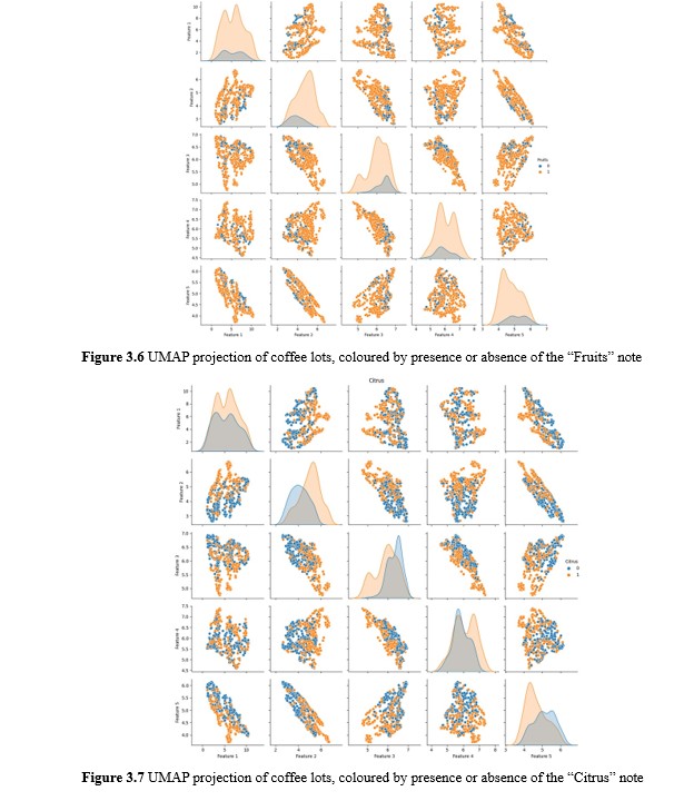
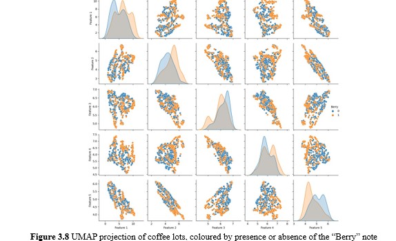
Perhaps expectedly, no notable discernible clusters emerged from UMAP projection. Closer inspection of the coloured labels revealed some interesting results however. An example of this is depicted in the UMAP plots for “Fruits”, “Citrus” and “Berries”. The SCA flavour wheel places “Citrus” and “Berries” as a subordinate flavour note under “Fruits”. Hence it was intriguing that this relationship could be discerned here, where the union of the datapoints with “Citrus” and “Berries” flavour notes almost perfectly corresponded with those exhibiting “Fruits”. Further, we observed that “Honey” and “Caramel” flavour notes appeared to be inverted, where a coffee that is described with “Honey” would be less likely to also be described with “Caramel”. Another noteworthy point is how samples with “Nuts” appeared to be a subset of those with “Cocoa”.
A caveat here to declare is the above observations were noted primarily with the consideration that the mentioned flavour notes were located adjacent in the flavour wheel - “Nutty” and “Cocoa” are adjacent under “Nutty/Cocoa” while “Honey” and “Caramel” are adjacent as well. Notwithstanding, these observations would later contribute to the decision of sub-chain ordering when we investigate modelling through classifier chains. A further conclusion on both PCA and UMAP is that whereas clear bias of categories were seen for multiple flavour notes, the separation of clusters is nevertheless poor. This foretells difficulties in subsequent modelling, save for the possibility that there could be clearer separations at higher dimensions since the visualisations presented above are two-dimensional.
Modelling
As described in an earlier section, four classification algorithms were considered in this work, namely, logistic regression, support vector classification, random forest, and AdaBoost. For each of these four algorithms, four pipelines were explored as well, creating 16 unique pipelines. The pipelines are tabulated as follows:
|
Preprocessing |
Dimensionality reduction |
Algorithm |
|
SNV |
PCA (2 - 23 components) |
Logistic regression (C: 0.001 - 100)
Support vector classification (rbf) (C, gamma: 0.001 - 1000) Random forest (n_estimators: 10-1000)
AdaBoost (n_estimators: 10-1000) |
|
nil |
||
|
SNV |
nil |
|
|
nil |
Gridsearch CV was conducted for all pipelines in order to choose the final pipeline with their respective relevant hyperparameters tuned based on the lowest Hamming loss. Based on the dataset, the baseline Hamming loss was calculated to be 0.3704 and the mean balanced accuracy is 0.5.
Binary Relevance
The binary relevance method settles on one best pipeline for each algorithm for all nine labels based on the pipeline and hyperparameters that yield the lowest mean cross validation Hamming loss calculated across all nine labels. The results are shown as follows:
|
Algorit hm |
Pipeline |
Hamming loss |
Mean balance d accurac y |
Balanced accuracy |
|||||||||
|
Train (CV) |
Test |
Floral |
Honey |
Caram el |
Fruits |
Citrus |
Berry |
Cocoa |
Nuts |
Spic e |
|||
|
Logistic Regres sion (LR) |
nil-nil-LR |
0.437 0 |
0.324 0 |
0.65 |
0.69 |
0.58 |
0.78 |
0.45 |
0.51 |
0.44 |
0.95 |
0.67 |
0.59 |
|
SVC |
nil-PCA- SVC |
0.351 5 |
0.379 6 |
0.48 |
0.50 |
0.67 |
0.50 |
0.50 |
0.43 |
0.51 |
0.50 |
0.33 |
0.37 |
|
Rando m Forest (RF) |
SNV-nil- RF |
0.352 2 |
0.351 8 |
0.52 |
0.44 |
0.50 |
0.39 |
0.50 |
0.46 |
0.69 |
0.50 |
0.58 |
0.59 |
|
AdaBoo st |
nil-PCA- AdaBoost |
0.403 4 |
0.453 7 |
0.49 |
0.44 |
0.50 |
0.28 |
0.45 |
0.31 |
0.59 |
0.86 |
0.67 |
0.34 |
Table 3.2 Modelling pipelines chosen for each classification algorithm with associated Hamming losses and balanced accuracies based on the binary relevance method.
Immediately, it is notable that logistic regression without any preprocessing nor dimensionality reduction performed the best on the test set despite having the poorest train metric (highest Hamming loss). Whereas the training set generated a Hamming loss higher than baseline, the test set Hamming loss was significantly lower. Conversely, the SVC pipeline which performed the best on the train set, came third with regards to the test set, slightly exceeding the baseline Hamming loss of 0.3704.
RF was the most appropriately fit algorithm, with both train and test metrics equivalent and better than baseline. This was also achieved without dimensionality reduction, indicating the ability of the RF algorithm in handling wide and short datasets robustly. AdaBoost surprisingly performed poorly even with the use of dimensionality reduction, performing poorer than baseline, and also showing signs of overfitting with a higher test Hamming loss than train despite the use of cross validation.
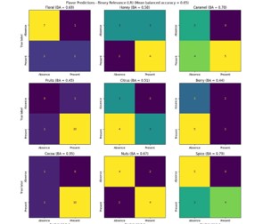
Figure 3.8 Confusion matrices of the nine flavour notes and their associated balanced accuracies (BA) for logistic regression
Inspecting the confusion matrices of the individual flavour notes as well as the balanced accuracy values in the above table provided some additional insights. Although “Floral”, “Fruits”, “Cocoa” were the most imbalanced, only “Fruits” underperformed the baseline balanced accuracy for the logistic regression model. In fact, “Floral” and “Cocoa” had among the highest balanced accuracies alongside “Caramel” and “Spice”. This observation however did not carry over to the other models. For example, the random forest model yielded balanced accuracies of 0.44, 0.5, 0.5 for “Floral”, “Fruits”, and “Cocoa” respectively. In general, what is obvious and expected is that all four algorithms work differently, generating results for the nine flavour notes that do not show any significant agreement amongst them.
Classifier Chain
As binary relevance reached 0.65 in mean balanced accuracy, the classifier chain approach was considered whereby it was believed that by using a preceding label to inform the next label being inferred, the overall performance could be improved. We started with a classifier chain, whereby the sequence was “Floral”, “Honey”, “Caramel”, “Fruits”, “Citrus”, “Berry”, “Cocoa”, “Nuts”, “Spice”. There was no particular meaning attached to the order; it was according to how the flavour notes were arranged on the Sweet Maria’s website. This would allow an inspection of the baseline performance of a classifier chain before any form of ordering or sub-chaining was employed. Selection of the best pipeline was done in a similar way to binary relevance, whereby one pipeline was chosen to represent all flavour notes based on the lowest mean Hamming loss across them.
|
Algorit hm |
Pipeline |
Hamming loss |
Mean balance d accurac y |
Balanced accuracy |
|||||||||
|
Train (CV) |
Test |
Floral |
Honey |
Caram el |
Fruits |
Citrus |
Berry |
Cocoa |
Nuts |
Spic e |
|||
|
Logistic Regres sion (LR) |
nil-nil-LR |
0.441 8 |
0.370 3 |
0.59 |
0.69 |
0.58 |
0.72 |
0.41 |
0.59 |
0.44 |
1.00 |
0.42 |
0.44 |
|
SVC |
nil-PCA- SVC |
0.359 5 |
0.407 4 |
0.46 |
0.50 |
0.58 |
0.50 |
0.50 |
0.24 |
0.51 |
0.50 |
0.50 |
0.27 |
|
Rando m Forest (RF) |
SNV-nil- RF |
0.359 2 |
0.342 8 |
0.54 |
0.44 |
0.50 |
0.56 |
0.45 |
0.36 |
0.69 |
0.50 |
0.75 |
0.59 |
|
AdaBoo st |
nil-PCA- AdaBoost |
0.403 4 |
0.472 2 |
0.44 |
0.44 |
0.25 |
0.56 |
0.41 |
0.31 |
0.54 |
0.5 |
0.5 |
0.49 |
Table 3.3 Modelling pipelines chosen for each classification algorithm with associated Hamming losses and balanced accuracies based on the classifier chain method.
Immediately, it is observable that the pipelines chosen for each of the four algorithms are exactly the same as they were for binary relevance. This suggests that the structure of the data consistently lends itself to certain pipelines, i.e. PCA preceding SVC is always preferred, perhaps because the transformation of the data into lower dimensional PCA space facilitates the separation of the classes more. Conversely, RF appears to work best with the full untransformed feature set, albeit with preprocessing to align the spectra first.
There was generally a notable abrogation in performance across the board; Hamming losses were all slightly increased from their binary relevance counterparts, and balanced accuracy also decreased with the sole exception of the RF pipeline. It appears that using the prior predictions to inform subsequent predictions was detrimental. We surmised two explanations for this phenomenon. First, it could be that the flavour notes were entirely unrelated, and using one to inform the other introduces noise instead. Second, it could be due to the specific sequence of the present classifier chain; the chain could have been incidentally ordered in a manner that caused any wrong predictions made earlier in the chain to carry forward the predictions down the chain. Indeed, we observed precipitous drops in balanced accuracies for “Citrus” in the SVC pipeline from 0.43 to 0.24 and “Nuts” in the LR pipeline from 0.67 to 0.42. With these findings, we moved on to an ordered classifier chain approach.
Ordered Classifier Chain
With regards to ordering the classifier chain sequence, we revisited the results from binary relevance. The hypothesis here was that by sequencing the classifier chain in descending order of the average mean balanced accuracies across all algorithms, the model would carry forward fewer errors and also benefit from a better fitted flavour note further up the chain to inform those down the chain. The order was determined as “Caramel”, “Nuts”, “Cocoa”, “Spice”, “Floral”, “Honey”, “Berry”, “Fruits”, “Citrus”
|
Algorit hm |
Pipeline |
Hamming loss |
Mean balance d accurac y |
Balanced accuracy |
|||||||||
|
Train (CV) |
Test |
Floral |
Honey |
Caram el |
Fruits |
Citrus |
Berry |
Cocoa |
Nuts |
Spic e |
|||
|
Logistic Regres sion (LR) |
nil-nil-LR |
0.434 9 |
0.462 9 |
0.66 |
0.62 |
0.67 |
0.78 |
0.36 |
0.59 |
0.54 |
0.91 |
0.67 |
0.76 |
|
SVC |
nil-PCA- SVC |
0.360 7 |
0.518 5 |
0.42 |
0.50 |
0.42 |
0.50 |
0.50 |
0.24 |
0.51 |
0.50 |
0.33 |
0.27 |
|
Rando m Forest (RF) |
SNV-nil- RF |
0.359 2 |
0.444 4 |
0.50 |
0.38 |
0.42 |
0.50 |
0.45 |
0.36 |
0.61 |
0.50 |
0.67 |
0.59 |
|
AdaBoo st |
nil-PCA- AdaBoost |
0.405 0 |
0.472 2 |
0.45 |
0.50 |
0.42 |
0.56 |
0.41 |
0.63 |
0.41 |
0.50 |
0.33 |
0.31 |
Table 3.4 Modelling pipelines chosen for each classification algorithm with associated Hamming losses and balanced accuracies based on the classifier chain method.
On first glance, we see that the test Hamming loss has increased across all algorithms, and it would appear that there is evidence of overfitting as well, as the train Hamming losses are all significantly lower than corresponding test values. Surprisingly, the balanced accuracies remained unaffected, if not improved; notably, the balanced accuracy for LR rebounded to 0.66, nearly matching that achieved with binary relevance. Through scrutinizing the metrics' computations, it becomes evident that the preservation or even enhancement of mean balanced accuracy values, coupled with a rise in Hamming losses, signifies a shift in mispredictions towards the majority classes rather than the minority ones. Notwithstanding, it is acknowledged that ordering the classifier chain in this method did not help with the overall model performance despite chaining the higher performing flavour notes upstream.
The above observations led to the question of whether chaining the flavour notes by their expected relationships would yield better results through exploitations of their inherent correlations. We explore this in the form of sub chains next.
Sub Chains
Based on the relationship between the flavour notes with reference to the flavour wheel above, the flavour notes were chained as follows:
|
Sub Chain |
Reason |
|
Honey → Caramel |
“Honey” and “Caramel” are adjacent on the outermost wheel in the innermost “Sweet” category. |
|
Fruits → Citrus → Berry |
“Citrus” and “Berry” belong to the second wheel in the innermost “Fruits” category |
|
Floral |
Standalone |
|
Spice |
Standalone |
|
Nuts → Cocoa |
“Nuts” and “Cocoa” are adjacent on the second wheel in the innermost “Nutty/Cocoa” categor |
Table 3.5 Sub chains and their respective rationales.
For each algorithm, the sub chains were optimised based on Hamming loss to yield the best pipeline, and the final train and test metrics were subsequently calculated based on predictions using a simple ensembling of the five sub chains. As a results, while every sub chain in one experiment would terminate in the same algorithm, the preprocessing pipelines may differ.
|
Algorith m |
Hamming loss |
Mean balance d accurac y |
Balanced accuracy |
|||||||||
|
Train (CV) |
Test |
Floral |
Honey |
Caram el |
Fruits |
Citrus |
Berry |
Cocoa |
Nuts |
Spice |
||
|
Logistic Regressi on (LR) |
0.4905 |
0.444 4 |
0.49 |
SNV- PCA |
nil-PCA |
nil-nil |
nil-nil |
nil- PCA |
||||
|
0.19 |
0.58 |
0.22 |
0.45 |
0.53 |
0.51 |
0.95 |
0.67 |
0.34 |
||||
|
SVC |
0.3345 |
0.379 6 |
0.47 |
nil-PCA |
nil-PCA |
nil-PCA |
nil-PCA |
nil-nil |
||||
|
0.50 |
0.50 |
0.50 |
0.50 |
0.36 |
0.51 |
0.50 |
0.33 |
0.50 |
||||
|
Random Forest (RF) |
0.3387 |
0.388 8 |
0.47 |
nil-SNV |
SNV-PCA |
SNV-PCA |
nil-nil |
nil-nil |
||||
|
0.44 |
0.42 |
0.50 |
0.50 |
0.43 |
0.59 |
0.50 |
0.50 |
0..31 |
||||
|
AdaBoost |
0.3872 |
0.472 2 |
0.43 |
nil-PCA |
nil-nil |
SNV-nil |
nil-PCA |
nil- PCA |
||||
|
0.44 |
0.42 |
0.44 |
0.41 |
0.39 |
0.44 |
0.50 |
0.42 |
0.44 |
||||
Table 3.6 Modelling pipelines chosen for each classification algorithm and sub chain with associated Hamming losses and balanced accuracies.
Surprisingly, the performance of the models when employing sub chains showed notable degradations across the board. Logistic regression, which has heretofore yielded mean balanced accuracies of above 0.50, now fared poorly at 0.49, alongside increased Hamming losses. In fact, some flavour notes such as “Floral” and “Caramel” had balanced accuracies of 0.19 and 0.22 respectively. The other algorithms did not fare well either, for example “Citrus” had a balanced accuracy of 0.63 for AdaBoost under an ordered classifier chain, but yielded 0.39 now when placed in a “Fruits” sub chain.
It would appear that the classifier chain approaches produce poorer results with increased complexity, with the sub chain approach being the worst despite supposedly being able to exploit inter label dependencies. The opportunity for each of the sub chains to optimise their individual pipelines also did not salvage the situation.
Decomposed Approaches
As evidenced by the series of classifier chain approaches producing increasingly worse results, our attention was turned towards approaches with lower complexity. For the decomposed approaches, two approaches were attempted. The first approach involved the independent training of nine binary classifiers, each for one flavour note. Each training session involved the selection of the best of all 16 different pipelines through maximising the cross validation balanced accuracy. The second approach involved extracting the pipeline that yielded the lowest cross validation Hamming loss for each flavour note in the binary relevance experiment. This limited the choice of pipelines to the four pipelines - nil-nil-LR; nil-PCA-SVC; SNV-nil-RF; and nil- PCA-AdaBoost.
|
|
Independently Trained Binary Classifiers |
Extracted From Binary Relevance |
|||
|
Flavour Note |
Pipeline |
Train CV Balanced Accuracy |
Test Balanced Accuracy |
Pipeline |
Test Balanced Accuracy |
|
Floral |
SNV-nil-SVC |
0.74 |
0.63 |
nil-nil-LR |
0.69 |
|
Honey |
SNV-PCA-RF |
0.65 |
0.50 |
nil-PCA-SVC |
0.67 |
|
Caramel |
nil-PCA-AdaBoost |
0.71 |
0.61 |
nil-nil-LR |
0.78 |
|
Fruits |
nil-nil-LR |
0.74 |
0.50 |
nil-PCA-SVC |
0.50 |
|
Citrus |
SNV-PCA-RF |
0.67 |
0.51 |
nil-nil-LR |
0.51 |
|
Berry |
SNV-AdaBoost |
0.74 |
0.76 |
SNV-nil-RF |
0.69 |
|
Cocoa |
PCA-AdaBoost |
0.76 |
0.45 |
nil-nil-LR |
0.95 |
|
Nuts |
SNV-PCA-RF |
0.71 |
0.67 |
nil-nil-LR |
0.67 |
|
Spice |
SNV-nil-AdaBoost |
0.65 |
0.71 |
nil-nil-LR |
0.79 |
|
|
|
Mean Balanced Accuracy |
0.59 |
Mean Balanced Accuracy |
0.69 |
|
|
|
Hamming Loss |
0.2963 |
Hamming Loss |
0.2778 |
Table 3.7 Model pipelines chosen for each flavour note when independently trained as binary classifiers and when extracted from binary relevance experiments.
At the expense of extensive computation, when we reverted to the most straightforward concept of framing the multilabel classification problem as a series of independent binary classifiers, the Hamming loss plunged to 0.2963. Meanwhile, the mean balanced accuracy only rose up to 59%, still lower than the 65% achieved with binary relevance using logistic regression without any form of preprocessing. On inspection of the train and test balanced accuracies, we also observed clear overfitting for almost all of the flavour notes, especially “Cocoa”. It would appear that by enforcing one single pipeline for all nine flavours in binary relevance, the propensity to overfit was reduced significantly. To show that this was indeed the case, we set up another alternative approach by extracting the pipelines from the binary relevance experiments corresponding to the best test balanced accuracy values for each flavour note. Here, we achieved a mean balanced accuracy of 69% alongside a respectable Hamming loss of 0.2778, which are the best metric values encountered thus far in this work. The agreement between a low Hamming loss and a high balanced accuracy also indicates that the mispredictions are neither biased towards the majority nor minority classes.
Discussion and Conclusion
This study investigated the use of multi-label classification using visible-NIR spectral data to simultaneously predict the flavour profiles of green coffee beans. We explored various multi-label classification approaches, including binary relevance, classifier chains, and decomposed methods. The second decomposed approach, where each flavour note was treated with its best- performing binary model from the binary relevance experiments, achieved the best results with a Hamming loss of 0.2778 and a mean balanced accuracy of 69%. It was possible that by extracting pipelines from the binary relevance experiments, the models were unintentionally regularised through prioritising overall performance, possibly reducing overfitting and leading to better overall metrics. Further, models for imbalanced flavours like "Floral" and "Cocoa" performed well, indicating the presence of distinct spectral signatures associated with these flavours, and this warrants further investigation (although not explored in this work). On the other hand, training the binary classifiers independently achieved a decent Hamming loss, but its mean balanced accuracy suffered (59%). This was likely due to overfitting in the small dataset (48 training samples, 12 test samples).
Classifier chain approaches yielded disappointing results, consistently performing below baseline. This was unexpected considering the premise of exploiting flavour note dependencies. The poor performance suggests either significant error propagation within the chains or that the flavour wheel relationships may not directly translate to the human tasting experience (e.g., tasting "Honey" doesn't necessarily imply "Caramel"). Alternatively, this could also be the effect of a small dataset. Further investigation into flavour note correlations could inform future chain design.
Notwithstanding the practical reasons that resulted in the procurement of only a small dataset, the present study demonstrates the potential of using visible-NIR spectroscopy for non-specific analysis to predict the flavour profiles of green coffee beans. Importantly, it suggests that especially for small datasets, it is safer to assume independence between the flavour labels. Future studies with larger datasets encompassing more tasters and a broader range of flavours on the flavour wheel could further refine these techniques. Additionally, a deeper investigation into flavour note correlations could inform the design and improvement of classifier chain approaches. Overall, this work provides a foundation for further research in predicting coffee flavour profiles through spectral analysis.
References
- Specialty Coffee Association. (2020). Coffee Flavor Wheel.
- Caporaso, N., Whitworth, M. B., & Fisk, I. D. (2022). Prediction of coffee aroma from single roasted coffee beans by hyperspectral imaging. Food chemistry, 371, 131159.
- Esteban-Díez, I., González-Sáiz, J. M., & Pizarro, C. (2004). Prediction of sensory properties of espresso from roasted coffee samples by near-infrared spectroscopy. Analytica Chimica Acta, 525(2), 171-182.
- Chang, Y. T., Hsueh, M. C., Hung, S. P., Lu, J. M., Peng, J. H., & Chen, S. F. (2021). Prediction of specialty coffee flavors based on nearâ?infrared spectra using machine and deepâ?learning methods. Journal of the Science of Food and Agriculture, 101(11), 4705-4714.
- Read, J., Pfahringer, B., Holmes, G., & Frank, E. (2011). Classifier chains for multi-label classification. Machine learning, 85, 333-359.
- Huang, J., Romero-Torres, S., & Moshgbar, M. (2010). Raman: practical considerations in data pre-treatment for Nir and Raman spectroscopy. American pharmaceutical review, 13(6), 116.
- Pedregosa, F., Varoquaux, G., Gramfort, A., Michel, V., Thirion, B., Grisel, O., ... & Duchesnay, É. (2011). Scikit- learn: Machine learning in Python. the Journal of machine Learning research, 12, 2825-2830.
- Becht, E., McInnes, L., Healy, J., Dutertre, C. A., Kwok, I. W., Ng, L. G., ... & Newell, E. W. (2019). Dimensionality reduction for visualizing single-cell data using UMAP. Nature biotechnology, 37(1), 38-44.
- Hsu, C. W., & Lin, C. J. (2002). A comparison of methods for multiclass support vector machines. IEEE transactions on Neural Networks, 13(2), 415-425.
- Hastie, T., Rosset, S., Zhu, J., & Zou, H. (2009). Multi-class adaboost. Statistics and its Interface, 2(3), 349-360.
- Zhang, M. L., Li, Y. K., Liu, X. Y., & Geng, X. (2018). Binary relevance for multi-label learning: an overview. Frontiers of Computer Science, 12, 191-202.
- Read, J., Pfahringer, B., Holmes, G., & Frank, E. (2021). Classifier chains: A review and perspectives. Journal of Artificial Intelligence Research, 70, 683-718.