

Journal of Electrical Electronics Engineering(JEEE)
ISSN: 2834-4928 | DOI: 10.33140/JEEE
Impact Factor: 1.2


Research Article - (2026) Volume 5, Issue 6
Emergent Quantum Mechanics - How the Classical Laws Can Mimic Non-Local (“Spooky”) Interactions
Received Date: Oct 02, 2026 / Accepted Date: Nov 09, 2026 / Published Date: Nov 19, 2026
Copyright: ©2026 Theo Van Holten. This is an open-access article distributed under the terms of the Creative Commons Attribution License, which permits unrestricted use, distribution, and reproduction in any medium, provided the original author and source are credited.
Citation: Holten, T. V. (2026). Emergent Quantum Mechanics - How the Classical Laws Can Mimic Non-Local (“Spooky”) Interactions. J Electrical Electron Eng, 5(6), 01-26.
Abstract
In Feynman’s “Lectures on Physics” it is observed that close to an oscillating dipole the electromagnetic field is almost quasi-static, as if retardation is absent and the speed of transmission thus would approach infinity. Within the framework of Emergent Quantum Mechanics (Em.QM) non-singular electron models are being revisited, showing similar phenomena near a droplet of charge. In the literature the matter has been called an as yet unsolved dilemma because – like the “spooky” non-local effects of Quantum Mechanics (QM) – it seems to be in conflict with relativity theory. In the present paper an asymptotic expansion of the electromagnetic field around a moving and deforming droplet of charge is used to investigate the matter in detail. It is concluded that Feynman’s formulae are correct, be it after initial conditions of the boundary value problem have been established by a field of normal traveling waves. When such a reset has been completed the field of traveling waves can be written as a superposition of groups of standing waves. In each standing wave system the variables belonging to it display synchronicity, which causes the illusion of non-retarded interactions. But in fact there are no causal relations between the singularities (such as charges) and the other field variables (such as electromagnetic forces), even though the illusion may be given that superluminal signalling takes place. The conclusions are important for the theory of Em.QM, since they show that the classical laws are able to mimic non-local phenomena.
Keywords
Emergent Quantum Mechanics, Droplet Model, Non-Retarded ("Spooky") Interactions, Non-Local PhenomenaIntroduction and Overview
In his Lectures on Physics, Feynman points out a remarkable and somewhat puzzling fact about the electromagnetic forces close to an accelerating charge or an oscillating dipole [1]. To quote Feynman: “Eq.......... gives [force] fields very much like the instantaneous theory – much closer than the instantaneous theory with a delay; ..........The static formulas are very accurate, much more accurate than you might think. Of course, the compensation only works for points close in“. In Feynman’s formulae the frequency of the oscillating dipole is unrestricted; the quasi-static phenomenon is therefore not associated with a low-frequency approximation.
The physical character of this near field region, in antenna theory called the “reactive near field”, is clearly seen when the flows of energy are analysed (see e.g. the calculation of the Poynting vector around a moving and deforming collection of charges in ref.2) [2]. At large distances one finds a smooth field, where a superposition of running waves carries energy away to infinity, in agreement with Larmor’s law. Closer in, orders of magnitude more intense flows of energy “slosh around” without contributing to the radiation at infinity. A visualisation of this kind of radiation field is the fierce turmoil in a pond beneath a waterfall, from which at some distance a smooth wave pattern emanates. It is in this highly disturbed near field that according to Feynman an unexpectedly small retardation of electromagnetic interactions occurs, much smaller than the ratio “distance of a field point from the point of emission divided by speed of light” would imply. It would seem as if the speed of interactions is superluminal (i.e. the kind of interactions Einstein called “spooky”). After mathematically analysing this curious near field phenomenon, Feynman alas did not philosophise further about possible physical interpretations, at least not in the “Lectures”.
Later, Walker (ref.3) performed experiments in the near field of a dipole antenna and discussed a few possible interpretations of the measured quasi-static phenomenon [3]. If one would accept that superluminal propagation is indeed possible, there is clearly a conflict with relativity theory. Relativity theory predicts that if an information signal is propagated superluminally, then it can be reflected by a moving frame and arrive at the source before the information was transmitted, thereby violating causality. Consequently, Einstein in 1907 stated that superluminal signal velocities are incompatible with relativity theory. Another possible interpretation mentioned by Walker is that there is a superluminal illusion caused by the fact that the near field could be a type of standing wave system, as suggested by the fact that high intensity flows of energy leave the source region and - since they for the most part do not reach infinity - must subsequently return. The system would thus largely consist of a field which grows and collapses synchronised with the oscillation of the electric dipole. This hypothesis was rejected by Walker on the grounds that the analysis in refs.3 and 4 does not show up such a standing wave system. Walker in ref.4 therefore states: “at present it is unclear how to resolve this dilemma” [4].
It is one of the goals of the present paper to revisit the latter “illusion interpretation”. In the paper the near field is derived in slightly more detail compared with Feynman’s and Walker’s field of a variable point-dipole. A point singularity is a mathematical idealisation of a physically more complex situation. Therefore, going back to the physical origin of the dipole model can give additional insight. Recently another case of non-retarded interactions has been found in the so-called “droplet theory” of Emergent Quantum Mechanics (hereafter abbreviated as Em.QM). It is this theory that is able to provide more details of the electromagnetic field than can be found in Feynman’s book. The present paper therefore first of all introduces and summarises the droplet theory of Em.QM.
The terminology “Em. QM” is here used for the theory describing cases where the classical laws can replicate the results of usual Quantum Mechanics (see refs.5, 6, 7) [5-7]. The aim of Em.QM is certainly not to compete with QM as far as practical calculations are concerned. However, Em.QM could become a complementary theory of QM, helping to obtain interpretations of quantum phenomena that are less “magical” than current ones, and – more importantly- to get causality back in the atomic world.
The droplet theory of Em.QM is based on the idea that a suitable theoretical model of electrons should include the inherent “zitter” motion. Time-averaging then leads to a non-singular electron model consisting of a deformable charge distribution, contained by surface-tension-like forces. The latter are non-physical “apparent” forces, only belonging to the time-averaged model world, and necessary as modelling additions to cancel the unrealistic “explosion forces” that artificially have been introduced by the time averaging. The background of this so-called “droplet model” is further described in refs.5, 6 and 7 [6,7]. Using the droplet model, the basic QM-laws E = hν and p = h/λ can be reproduced by the classical laws, whilst a practically correct value of Planck’s constant h is found. Other results of the droplet theory include a full replication of the quantum harmonic oscillator (ref.7), and (in ref.6) a possible solution of the long-standing “enigma” of the muon and tau-particle (why do three “generations” of leptons exist, and how can the corresponding mass differences between them be explained?).
A non-uniformly moving and deforming charge distribution as considered in the droplet theory is always subjected to so-called electromagnetic self-forces, arising by internal retardation effects (ref.8). On a non-deforming charge distribution, as originally investigated by Lorentz (ref.9) and more recently by Yaghjian (ref.10), two self-forces act: an inertia force associated with so-called “electromagnetic mass”, and radiation resistance [8-10]. The extra feature of droplet theory is, that it requires the determination of self-forces on a lump of charges which changes its shape, apart from its translational motion. The tool used in this case for determining the associated electromagnetic field is the “matched asymptotic expansion” technique (hereafter abbreviated as “max” method). The method uses local “coordinate-stretching” in the vicinity of singularities and enables one to determine the field inside and outside charge distributions in detail, as if seen through a (mathematical) microscope. Here again, the same seemingly superluminal phenomena as mentioned by Feynman are found, be it that more details can be discovered.
The present paper has a twofold aim. The first is, to more deeply investigate the phenomenon of non-retarded interactions: how they can be consequences of Maxwell’s laws, and how they might be reconciled with relativity theory.
Secondly, the subject of the present paper has direct and important consequences for Em.QM in general. In spite of past successes, it is often said that Em.QM will always be limited in its scope because “it is believed that the classical laws never will be able to replicate non-local effects (i.e. events causing a remote effect without retardation) ”. Or in jargon terminology: any theory containing hidden variables must encompass "actio-in-distans", which -it is thought- excludes the classical laws from being candidates to offer a valid interpretation of quantum theory. This opinion was in the past already contradicted in a paper by Anderson and Brady (ref.11), where the authors showed that a certain type of classical system can satisfy the so-called Bell test, which test is able to prove the existence of non-local effects [11]. If the occurrence of non-retarded interactions as found by Feynman and Walker as well as in the ”droplet theory” can be ascertained beyond doubt and physically explained, this would show that Em.QM is not fundamentally barred from covering the whole of QM.
Until now the results of the droplet theory have been obtained by using the simplest possible model of a deformable lump of charges. The limited aim so far has been to reconsider non-singular electron models and perform a first exploration to find the consequences of such models. For this reason a “minimum complexity” model has been adopted (figure1), consisting of a one-dimensional potential well in which a slender “droplet” of charge moves back and forth with so-called “pulsation” freedom (i.e. lengthwise stretching and contracting). In sec.2 the boundary value problem is formulated which has to be satisfied by the scalar and vector potentials associated with this kind of model.
The next sec.3 describes the principles of the “matched asymptotic expansion” technique, or “max”-method. The expansion parameter of the asymptotic series is the ratio a ⁄ λ, where a denotes a typical dimension of the potential well and the near field, and λ a typical wavelength in the far field. For small a ⁄ λ the potentials in the near field can be written as quasi-static fields augmented by an asymptotic series. On the other hand, in the far field the limiting process a ⁄ λ→0 implies that the field may be approximated by a superposition of multipoles in the origin. Both the near- and far field approximations are not unambiguous because of missing boundary conditions either at infinity or near the origin respectively. This causes that the near field may contain fields that do not vanish at infinity, and that these additional fields even prove essential when determining the forces in the near field. “Matching” through the mediation of a so-called “common field” finally achieves an unambiguous “composite” solution which satisfies all the boundary conditions and where any singularities have been cancelled by the matching.
How the in sec.3 outlined “max” procedure can be applied in actual cases is illustrated in sec.4 , where the potential fields of a moving point charge are calculated, as well as the force field around it. In the theory of a moving and deforming droplet the contribution by infinitesimal elements of the droplet is integrated, using the point charge results (sec.5).
In this way an inertial self-force (usually expressed in terms of an “electromagnetic mass”) is found as well as the so-called radiation resistance, in agreement with Lorentz’s classical results. Both these self-forces are related without retardation to corresponding properties of the motion: the electromagnetic inertia is associated with the instantaneous acceleration, and the radiation resistance is proportional to the instantaneous jerk. It is only thanks to the non-retardation that the concept of electromagnetic mass can be introduced at all. Were it not so, then the value of electromagnetic mass would depend on the motion history of the droplet. The same is true for the radiation resistance self-force.
Also in sec.5 the non-retarded forces between separate droplets of charge are considered. A lump of charges is taken as an example, breaking up into two separate droplets. The pair of two fragments may be viewed as an extreme form of deformation. As long as the dimensions of the total constellation remain small compared with the wavelength of disturbances in the far field, both fragments share the same near field and interactions between them appear to be non-retarded.
A convergence investigation in sec.6 shows that the asymptotic series solution is entirely equivalent with a superposition of traveling waves if certain conditions are fulfilled. These requirements entail that the boundary conditions determining the field are smoothly evolving in time, without discontinuities in any of the time derivatives. A simple example would be a system of two droplets of charge, sharing a common near field, and sinusoidally closing in and moving away from each other under the influence of an external potential. If the requirement of continuity is not satisfied (for instance during the starting-up of a harmonic motion), during a short interval of time the asymptotic series do not converge to the correct value, and the only way to describe the field is by a superposition of traveling waves (with full retardation effects). During such a transient both new boundary conditions are being established as well as new initial conditions. After the "reset" the further development of the near field can be described again by an asymptotic series (including the phenomena of non-retarded electromagnetic forces).
How these findings can be interpreted physically, and how they can be reconciled with relativity theory is discussed in secs. 7 and 8. It is shown that the complete asymptotic series, equivalent with the field of traveling waves, can be separated into a superposition of standing waves. In case the boundary conditions require a harmonically variable field, the variables belonging to one particular standing wave system are in phase throughout the field. This synchronous behaviour pertains to the entire standing wave system including any embedded singularities, but does not pertain to the variables belonging to another standing wave. The synchronous variation of the quantities belonging to a particular standing wave system does not imply an infinite speed of signal transmission from a singularity to a field point (as if a singularity could exist individually, and as if there would be a causal relation between the singularity and the field, such as incorrectly suggested by the common parlance about a "field induced by a charge"). The field, including its embedded singularities and force fields, develops as a whole, simultaneously in all points. This gives rise to the illusion of non-retarded interactions.
In the conclusions (sec.9) a further discussion about the significance of the findings is included. The dilemma “superluminal effects versus relativity” raised in the publications by Feynman (ref.1) and Walker (ref.4) would seem to be solved [1,4]. Furthermore, one may safely state that Em.QM indeed covers phenomena that may be called holistic, non-local or - in Einstein's words - “spooky”. However, prior to a future further development of the droplet theory to include "spin" it is not possible to compare these conclusions with the non-local phenomena known in the usual QM.
The Boundary Value Problem of the Droplet of Charge
The droplet model of electrons, depicted in fig.1, has its origin in the principle to model electrons including their “zitter” (“shudder” or “tremble”) motion, in such a way that the real physics become amenable to a reasonably simple, although approximate analysis. Another point of view, which will be taken here for the sake of brevity is, that one may propose any kind of model –however unrealistic it might seem at first sight- as long as the consequences agree with experiments. In this respect the droplet model has proven its value (see refs. 5, 6 ,7) [5-7].
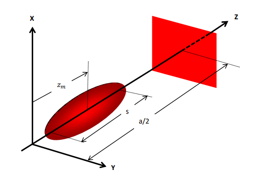
Figure 1: Notations Droplet In Potential Well
The model configuration analysed in these references consisted of a charge distribution contained by “surface-tension-like” apparent forces, moving back and forth along the Z-axis inside a two-dimensional potential well. The distribution has an elongated shape, with rotational symmetry around the Z-axis and furthermore symmetry w.r.t. an “equator-plane”. All of these model assumptions were introduced in order to simplify the mathematics and obtain quick and simple answers in an exploratory study whether non-singular electron models could make sense. The two degrees of freedom of this model were translation zm (t) of the midpoint (which is the centre of charge as well as the centre of mass), and the variable length s(t).
The (electric) scalar potential Φ(x, y, z, t) should satisfy the field equation

where σ(x, y, z, t) denotes the charge density. The (magnetic) vector potential A (X, Y ,Z, t) must satisfy a similar field equation where the current density j is on the r.h.s.:

In the free space outside the charge- and current distributions the scalar potential and the three Cartesian components (Ax , Ay , Az ) of 2 the vector potential satisfy wave equations such as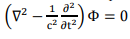 and are required to vanish at infinity.
Matched Asymptotic Expansion (Max) Analysis of the Non-Stationary Electromagnetic Field
Near-Field Approximation
When a “lump” of electrical charges is moving back and forth with some regularity along a stretch of the Z-axis, one can assign a characteristic time scale T to the motion. T can for instance denote the typical average duration to complete a cycle of the -not necessarily harmonic- motion. If the motion covers a variable length of the Z-axis characterised by a scale a, a characteristic velocity of the motion may be defined as v = a / T.
The region of space close to the stretch of the Z-axis where the motion takes place will be called the “near field”. It is a volume of space with global dimensions of the same order of magnitude a. Within this near field the spatial variations of the electrical potential Φ will have a scale of order a, or smaller. This strictly applies to the near field only, and will not be true in the whole of space stretching out to infinity. A typical length scale far away from the charge will be the wavelength λ = cT of electromagnetic waves associated with the moving charge, with c the speed of light. In the near field (outside the charges) the wave equation may be written in terms of the characteristic coordinates 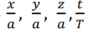 :

where all the partial derivatives in eq.(3) have the same order of magnitude, on account of the physical assumptions about the space- and time scales in the near field.
The basic assumption of the matched asymptotic expansion procedure is, that the ratio a / λ is small, so that it may be used as an expansion parameter in an asymptotic series developed for a/λ → 0. An equivalent expansion parameter is the ratio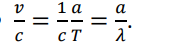
According to eq.(3) the field Φnear (x, y, z, t) in the limit a/λ → 0 will approach a quasi-static field Φqu.static satisfying the Laplace equation ∇2Φqu.static = 0 outside the distribution of charges. The terminology “quasi-static” is used to indicate that the field at any instant of time is spatially identical to the field of a static distribution of charges, even if the shape and strength of the charge distribution are functions of time. Changing boundary conditions thus lead to a time-sequence of static-like fields.
The quasi-static field is used as the first term in an asymptotic expansion, whilst the other terms of the series describe how the field is influenced by retardation effects:

To determine the equations that have to be satisfied by the additional fields Φ1, Φ2 ,… expression (4) is substituted into the wave equation (3):

As a next step ∇2 Φqu.static = 0 is subtracted from eq.(5) and the equation is divided by  Taking again the limit a/λ → 0 gives an equation which has to be satisfied by Φ1 , etc. The same results may be obtained by equating terms on the l.h.s. to terms of the same asymptotic order on the r.h.s. The procedure shows that up to and including the order
 the near field satisfies the following Poisson equation:

The solution of this Poisson equation again has the character of a spatially static-like field, now “induced” by a virtual distribution of sources and sinks, as specified by the r.h.s. of eq.(6). This virtual charge distribution covers the entire space, in contrast to the physical charges inducing Φqu.static .
Higher order approximations accurate up to and including the order  with n ≥ 4, will similarly obey the recurrence relations

from which it follows

where the notation (Φnear )n stands for the partial sum

When n is increased step by step, the “stack” of fields (Φnear )n , determined by eqs. (6) and (8), may be viewed as a sequence of successive approximations, calculated for a given time. If this sequence of approximations converges, i.e. if Φn → 0 and (Φnear )n-2 →(Φnear )n for n → ∞, then according to eq.(8) the converged field (Φnear )n→∞ exactly satisfies the original wave equation:

In sec.6 it is investigated under which –physically realisable- conditions convergence may be expected.
The conclusion is that, under conditions guaranteeing convergence, the solution of the wave equation can be formulated in two different but equivalent forms: either as a superposition of traveling waves, or alternatively as a series-expansion like eq.(4). The traveling wave solution shows the retardations explicitly, whereas the series-expansion is a cross-section for a given time, where time enters as a parameter only and retardation effects are not explicit. Of course, retardation effects are physical realities, but in the representation by an asymptotic series they are implicit: the effects of retardation are mimicked thanks to the presence of the r.h.s. of the Poisson equations (6) and (8).
To return to eq.(6), valid up to and including the order ,sec.4 will deal with its solution. The complete solution will consist of a particular solution of the Poisson equation, summed with appropriate solutions of the Laplace equation ∇2 Φnear = 0. The latter solutions of the homogeneous equation must anyway comprise the quasi-static field Φqu.static , whose singularities represent the physical charge distribution. However, the near-field approximation misses boundary conditions at infinity (because the derivation of the Poisson equation is valid in the near field only) so that another contribution to the near field  Φ is possible (and actually does occur), satisfying the Laplace equation ∇2 (Φ) = 0 and not necessarily vanishing at infinity. This additional field Φ cannot yet be determined because of the incompleteness of the boundary value problem. The ambiguity of the solution will be removed by so-called “matching” with a far-field approximation.