Duration vs. Catastrophe: A Survival-Based Decomposition of Financial Fragility via the Clock of Regimes Model*

Introduction

Conventional financial risk models are structurally fragile because they assume ergodicity and memoryless dynamics in environments characterized by fat tails and temporal asymmetry (Taleb, 2016). Gaussian diffusion frameworks treat volatility as stationary and independent across time, while standard Hidden Markov Models (HMMs) impose geometric residence times that underestimate duration clustering and persistent tail risk (Hamilton, 1989, 1990, 2016). These assumptions distort the temporal structure of exposure and systematically misprice ruin.

The Clock of Regimes (COR) model is a new class of regime-switching model characterized by the N = −K⁻¹ operator (Linares and Bulavas, 2026). Within a Talebian framework, fragility is excessive concentration of probability mass in adverse states over time (Taleb, 2016). The COR model formalizes antifragility by contracting exposure as hazard intensifies and redeploying convexity as stress dissipates. Tail probabilities become state-conditional objects weighted by survival structure instead of unconditional frequencies.

This paper implements the COR model, a novel duration-aware stochastic framework that extends classical HMMs by embedding survival and hazard calculus directly into regime-switching dynamics, by shifting the focus from one-step transition probabilities to a continuous-time operator N = −K⁻¹ (Berman and Shoenfeld, 1956; Hearon, 1972, 1981; Eisenfeld, 1981; Covell et al., 1984; Linares et al., 1987, 1988; Jacquez and Simon, 1993; Jacquez, 2002), we transform latent market states into a measurable temporal geometry of probability mass1. Using E-mini S&P 500 futures (ES) and S&P 500 index (SPX) historical market data, our study demonstrates that a Student-t HMM specification is statistically superior to Gaussian alternatives, uncovering a path-dependent market structure where steady regimes harbor hidden fragility and stress regimes act as high-intensity exit portals. The architecture culminates in a spectral fragility measure, which quantifies systemic risk not as a static probability, but as a structural leak of survival probability mass, ultimately providing a rigorous mathematical foundation for ruin-sensitive decision-making in nonlinear markets

Empirical Validation

Through comprehensive numerical experiments and comparative analysis, this section describes the empirical implementation of the COR model. The methodology combines heavy-tailed HMM estimation with survival-adjusted operator construction in order to quantify systemic fragility in financial return series of the E-mini S&P 500 futures (ES) and the S&P 500 index (SPX).

Data and Return Construction

Let denote an observed asset price series sampled at a fixed frequency. Log returns aredefined as

In this study, the COR analysis is conducted on historical daily return data. All datasets used in the empirical comparison are aligned in sample length to ensure structural comparability of regime estimates and operator-based risk metrics.

Hidden Markov Model Specification

We assume that returns follow a finite-state Hidden Markov Model with K latent regimes. Conditional on regime S_t = i , returns are distributed according to a Student-t distribution:

Likelihood and Estimation

Parameters were estimated by maximum likelihood using the Expectation–Maximization algo¬rithm (Baum et al., 1970). The E-step computes filtered and smoothed regime probabilities using the forward–backward recursion in log scale to ensure numerical stability. The M-step updates transition probabilities, regime means, and scale parameters using smoothed sufficient statistics. Degrees of freedom are estimated via profile likelihood or grid search to improve convergence robustness.

After estimation, regimes are reordered according to increasing conditional variance in order to obtain an economically interpretable state ordering from calm to crisis.

Hazard Calibration

To incorporate survival dynamics, a regime-dependent hazard rate is assigned using a tail-sensitive mapping:

where ensures structural openness and C > 0 controls sensitivity to tail thickness. This rule captures the intuition that regimes with heavier tails exhibit higher systemic leakage risk.

Operator Construction

Given the estimated transition matrix A  and hazard vector the open transition operator is constructed as

The generator is then defined as                  K = Q − I,

and the fundamental matrix                       N = −K⁻¹

is computed numerically and interpreted as the expected survival-weighted residence time across regimes.

Residence Distribution

A survival-weighted regime distribution is derived from the leading left eigenvector of Q, normalized to sum to one. This vector provides the long-run allocation of temporal probability mass across regimes under open-system dynamics.

Tail Risk Measurement

For each regime, the left-tail probability at level is computed using the fitted Student-t distribution:

Aggregate tail exposure is defined as the residence-weighted average

Structural Ruin Metrics

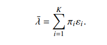
Average hazard leakage is computed as,

Given a risk horizonT_h, a structural ruin probability bound is obtained via

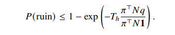
This metric integrates regime persistence, tail severity, and systemic openness into a unified survival-oriented risk measure.

Rolling Estimation

To study time variation in systemic fragility, the entire estimation procedure can be implemented on rolling windows of fixed length. This produces time series of regime probabilities, operator spectra, and ruin metrics, allowing early-warning monitoring of structural market instability.

The empirical methodology therefore deploys the theoretical COR model by combining heavy-tailed regime estimation with operator-based survival analysis, yielding tractable measures of persistence fragility, catastrophe fragility, and ruin exposure.

Data Source

The daily historical data for analysis was sourced via Yahoo Finance (Yahoo, 2026), which provides a robust and accessible foundation of historical data for both the ES (E-mini S&P 500 Futures) and the SPX (S&P 500 Index) time series. By utilizing closing prices, the model ensures that the calibration of daily paths remain anchored to widely recognized market benchmarks. This data allows for the precise mapping of regime transitions and the calculation of probability mass across the 2007–2009 epoch, capturing the high-fidelity volatility signatures required for the Clock of Regimes model.

The E-mini S&P 500 (ES) is a highly liquid futures contract traded on the Chicago Mercantile Exchange (CME) (CME Group Inc., 2026). ES is a derivative of the underlying S&P 500 index. Represented by tickers such as ES or ES=F, it allows traders to control a significant notional value—calculated as $50 times the current index level—through the use of margin-based leverage. A primary advantage of the ES is its nearly 24-hour trading session, providing continuous price discovery and liquidity far beyond standard equity market hours. E-mini S&P 500 (ES) futures trade on CME Globex, running from Sunday to Friday, 6:00 p.m. to 5:00 p.m. ET, with a daily 1-hour maintenance break at 5:00 p.m. ET. The most liquid times are during regular U.S. trading hours (9:30 a.m. – 4:00 p.m. ET). Because of its capital efficiency and round-the-clock access, the instrument is a cornerstone for professional macro speculation, high-frequency short-term trading, and institutional hedging strategies designed to offset broader equity portfolio risk.

The S&P 500 Index (SPX) is a market-capitalization-weighted index of 500 of the largest publicly traded companies in the United States (Cboe Exchange, 2026). Represented by tickers such as SPX or ^GSPC, SPX is a theoretical benchmark—a cash index—that cannot be traded directly; instead, investors gain exposure to it through exchange-traded funds (ETFs) like the SPY or through settled option contracts. CBOE SPX options are European-style, cash-settled contracts based on the S&P 500 Index, trading under the ticker SPX ($100 multiplier). Standard SPX options expire monthly (3rd Friday), while SPX Weeklys (SPXW) expire daily/weekly, offering high liquidity for broad market hedging without physical delivery or early assignment. SPX options trade during Regular Trading Hours (RTH) from 9:30 a.m. to 4:15 p.m. ET, Monday-Friday, with added liquidity during Global Trading Hours (GTH) from 8:15 p.m. to 9:25 a.m. ET. Expiring SPX Weeklys (SPXW) often close at 4:00 p.m. ET on their expiration day, with overnight close sessions available. SPX serves as the primary gauge for the health of the U.S. equity market and is the underlying reference for a vast ecosystem of financial derivatives. SPX remains the definitive anchor for long-term valuation, academic benchmarking, and institutional performance measurement.

Methods

The Clock of Regimes Model

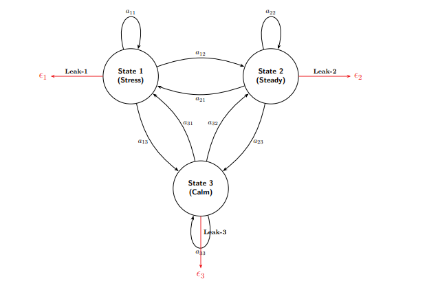
                   Figure 1: The Clock of Regimes model architecture.

This section develops the theoretical structure of the COR model (Figure 1). The COR model interprets regime switching as an open dynamical system whose temporal evolution determines the accumulation of systemic risk. Unlike standard HMM approaches that focus primarily on classification or persistence, the COR model emphasizes survival geometry and the temporal probability mass within adverse market states.

The COR model (Figure 1) classifies market behavior into three distinct states (The Nodes) to track shifting dynamics. State 1 (Stress) is identified as an intermediate or heightened-risk environment where volatility begins to expand and the system moves away from its baseline. State 2 (Steady) represents the normal or equilibrium state of the system, characterized by standard liquidity and predictable price action. Finally, State 3 (Calm) denotes the most favorable, low-volatility environment where market participants experience maximum stability and minimal systemic friction. Each node features a self-loop arrow, which visually represents the diagonal entries of the transition matrix A (or the self-persistence in the generator matrix K). This indicates the probability of the system remaining in its current state during a discrete time step.

The COR model maps the transitions between market environments through three primary interaction paths. The State 1 ↔ State 2 path represents the escalation/de-escalation phase, where the system oscillates between heightened stress and a steady, equilibrium condition. The State 2 — State 3 path covers the normalization/improvement phase, tracking the shift between a steady market and a low-volatility, calm environment. Finally, the State 1 ↔ State 3 path accounts for direct transitions, capturing extreme market phenomena such as flash crashes or rapid V-shaped recoveries where the system bypasses the steady-state intermediary entirely.

Regime Dynamics

Let {S _t} t ≥0 denote a finite-state Markov chain with state space {1, . . . , K} and transition matrix A. The latent state governs the conditional distribution of asset returns, which may exhibit heavy-tailed behavior. In empirical applications, we allow regime-dependent Student-t  emissions to capture discontinuous market shocks.

The Transition Probability Matrix A

The transition matrix A describes closed-system regime dynamics. However, financial systems are inherently open: adverse events may trigger structural exits such as systemic liquidation, default cascades, or market shutdown. To incorporate this feature, we introduce a regime-dependent hazard vector

Hence, the A matrix governs the evolution of the system over a discrete time step 

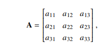
where the conservation of probability mass for each state i is defined by the specific leakage

Open Transition Operator

The hazard-adjusted transition operator is defined as

The matrix Q is substochastic, reflecting the possibility of absorption outside the modeled regime system. This construction converts the regime-switching process into an open Markov system whose evolution tracks survival-weighted probability mass.

Continuous-Time Limit

To analyze temporal exposure, we consider the generator

                                                                            K = Q − I,

which can be interpreted as a discrete-time approximation to a continuous-time Markov generator. This result establishes a bridge between discrete HMMs and continuous-time survival processes via the generator K matrix,

Fundamental Matrix and Survival Geometry

The fundamental matrix of the open system is

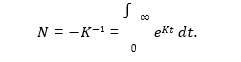
The element N_{i j} represents the expected survival-weighted time spent in regime j when starting from regime i. Thus N provides a direct measure of temporal probability mass. In financial terms, large diagonal entries of N indicate durational entrapment in adverse regimes, while large off-diagonal entries reveal conduit states through which systemic fragility propagates.

The Fundamental Matrix (N = −K⁻¹) may be derived by inverting the negative of the K matrix (Hearon, 1972, 1981; Eisenfeld, 1981; Covell et al., 1984; Linares et al., 1987, 1988; Jacquez, 2002). The inverse of this matrix calculates the expected Persistence of Probability Mass (Residence Time) within each of the nodes (Figure 1)—essentially, how much total time the market spends in a specific regime before it eventually leaks out or transitions.

Fragility Decomposition

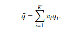
Let q_i denote the left-tail probability of returns conditional on regime i. Let .png denote the survival-weighted regime distribution derived from N . Define the residence-weighted tail exposure,

Similarly define the average hazard leakage as,

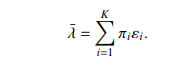
This decomposition formalizes the intuition that markets may be fragile either because they remain trapped in adverse regimes or because losses accumulate rapidly during crisis episodes. This result connects heavy-tailed shocks and regime persistence to operator-level measures of systemic risk.

Spectral Fragility Let

_P(N) denote the spectral radius of the fundamental matrix. An increase in _P(N) indicates expansion of survival-weighted residence time across regimes.

Residence-Weighted Ruin Bound

Let T_h denote a risk horizon. Define the structural ruin probability bound This bound captures the interaction between regime duration, tail exposure, and hazard structure.

Taken together, the COR model provides a unified operator-theoretic representation of financial fragility. It embeds heavy-tailed regime switching within survival dynamics and yields tractable measures of systemic exposure, persistence, and ruin risk.

Results

Data

The analysis focuses on daily historical data of E-mini S&P 500 Futures (ES) and the S&P 500 index (SPX) during the Global Financial Crisis crash from 2007 to 2009. The COR analysis is conducted on historical daily return data.Let denote an observed ES or SPX asset price series sampled at a fixed frequency. Log returns are defined as,

All datasets used in the empirical comparison are aligned in sample length to ensure structural comparability of regime estimates and operator-based risk metrics. The empirical analysis is based on datasets comprising 755 price observations, which translates into 754 log-return calculations for the ES and SPX time series. The essential COR model analysis is that the HMM layer identifies three economically distinct regimes, and the COR model layer then converts those local switching dynamics into a survival geometry through the Q K, and N matrices.

To capture the shifting market dynamics, the COR model identifies three distinct hidden regimes (Stress, Steady, and Calm). In the COR model, these states are not just descriptive labels; they are formalized mathematical environments defined by the interaction of drift volatility , and tail thickness (v) characterized by unique volatility and drift parameters. The tail risk is formally evaluated at a probability level of = 0.01, allowing the model to focus on extreme left-tail events that represent potential systemic failures. Finally, these structural parameters are integrated over a

ruin horizon of T = 250 trading days, providing a standardized one-year window to quantify the cumulative probability of wealth destruction or regime exit.

 Model Specification

For both ES and SPX, the structural evaluation of the COR model analysis involves a formal comparison between two competing model specifications: a standard Gaussian Hidden Markov Model (HMM) and a Student t Hidden Markov( Model t-HMM). While the Gaussian approach assumes normally distributed shocks within each regime, the Student-t specification explicitly accounts for the excess kurtosis often observed in ES and SPX returns during periods of systemic instability.

Findings for SPX

Empirically, the Student-t model demonstrates a statistically superior fit to the crash data, achieving a higher log-likelihood of  _Student = 2147.54 compared to _Gaussian = 2140.54 (Table 1). The substantial gain in the log-likelihood (+7.00) confirms that a heavy-tailed distribution is necessary to accurately capture the discontinuous price movements and flash volatility that define the catastrophe fragility channel.

To further quantify model performance, we evaluated the Akaike Information Criterion (AIC) and the Bayesian Information Criterion (BIC). These metrics provide a penalized assessment of the log-likelihoods, balancing the goodness-of-fit against the structural complexity of the model. As tablulated in Table 1, while the BIC slightly favors the Gaussian model due to its stricter penalty for the three extra degrees of freedom (K = 15), the AIC and Log-Likelihood confirm that the Student- t model provides a fundamentally better representation of the heavy tails in the E S and S P X return series.

Transition Dynamics

Gaussian Transition Matrix A : The Gaussian model identifies the following transition probabilities between the three identified regimes:

Student-t Transition Matrix A : The Student-t model, which provided a higher log-likelihood of 2147.54, identifies these switching dynamics:

In both models, the diagonal elements are all > 0.95, indicating high regime persistence where states are likely to remain the same from one day to the next. Both matrices show a 0.000000 probability of a direct jump between State 1 (Bull/Low Vol) and State 3 (Crisis/High Vol), suggesting the system must pass through the neutral State 2 to transition between extremes. The Student-t State 1 (0.9787) is more stable than the Gaussian State 1 (0.9608), which influences the subsequent COR generator K and the survival geometry of the model.

Hazard-Adjusted Survival Operator
The Hazard-adjusted survival operator Q serves as the core survival geometry within the COR model. It modifies the standard transition dynamics by accounting for the probability of emphescaping or failing to survive a regime.

Each row sum satisfies

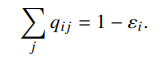
The matrix maintains a structural zero between State 1 and State 3, indicating that direct transitions between the extreme bull and crisis regimes are statistically impossible without passing through the intermediate State 2. Note that the row sums of Q are strictly < 1.

The COR Generator Matrix

The COR generator K matrix is derived directly from the hazard-adjusted transition operator Q  by the relation K = Q − I. This matrix represents the instantaneous rates of flow and leakage (risk) or hazard rate of each system state.

The diagonal elements of K represent the total exit rate from each state.  State 1 has the highest exit rate at −0.043292, indicating it is the most transient regime in this dataset. These values represent the rates of moving specifically from one regime to another. For example, the rate of moving from State 2 to State 1 is 0.015740. Unlike a standard Markov generator where rows sum to zero, these rows sum to a negative value. This missing probability mass is the local hazard rate, which the model uses to calculate the Residence-weighted hazard (^¯) of 0.014943.

The Fundamental Matrix

The Fundamental Matrix N = −K⁻¹ is the centerpiece of the COR model’s survival analysis. It translates the instantaneous flow rates of the generator into the expected number of days the system will reside in each state before leaking or failing.

The diagonal elements N_ii represent the total expected time spent in Statei i (State Persistence) given that the system started in State i. State 2 (Moderate Volatility) has the longest expected residence at 47.88 days, closely followed by State 3 (Crisis) at 45.66 days.

The off-diagonal elements show how much time one state contributes to another (Inter-Regime Support) before exiting the system. For instance, if the system starts in the Bull regime (State 1), it is expected to spend about 23 days in the Neutral regime (State 2) before eventually dying or hitting the ruin threshold. If the system starts in State 3, it only expects to spend 5.63 days in the safe State 1, highlighting the difficulty of escaping high-volatility regimes (Crisis Vulnerability) during the 2007–2009 period.

Summing the rows of N gives the total expected time until a ruin event occurs (Total Expected Life) for each starting state. For a system starting in State 2, the total life expectancy is approximately 72.07 days (17.41 + 47.88 + 6.77).

The State Summary

The State Summary provides the empirical parameters for each regime (Table 2), bridging the abstract matrix algebra of the COR model with the actual market behavior of the SPX from 2007–2009.

As tabulated in Table 2, State 1, the Low Volatility Bull State exhibits the highest positive drift and the lowest volatility. Interestingly, it has a low v = 4, indicating that even in good times, the returns had heavy tails. State 2, the Moderate/Gaussian-like, withv = 100, is effectively Gaussian. It represents a normal market state with near-zero drift and moderate risk. State 3 (High Volatility/Crisis, is characterized by extreme volatility (over 5× higher than State 1) and a significant negative drift. The expected spell of 132.14 days underscores the persistent nature of the 2008 financial collapse. State 3, Tail Risk ( and q _tail), carries a local tail probability ( q _tail)) of 0.0575, which is nearly 600% higher than the target = 0.01.

The COR model effectively aggregates these distinct states into a single, unified survival outlook for a 250-day trading horizon : the calculated Residence-Weighted Tail Probability (q¯) is 0.011956, which represents the average probability of a tail event occurring across the different regimes. This is complemented by a Residence-Weighted Hazard (^¯) of 0.014943, reflecting the integrated risk of "leaking" out of a stable state into a ruin event. Ultimately, for a horizon of T = 250, the model establishes a Ruin Bound of 0.043681, indicating approximately a 4.37% probability of the system failing to survive the specified threshold over the course of a trading year

 Regime Characteristics

The SPX COR analysis reveals a market structure characterized by a three-state regime architecture (Table 3).

State 1: Crisis (The “Systemic Rupture” Regime)

• Description: The Crisis regime is a non-ergodic state where standard valuation models break down.

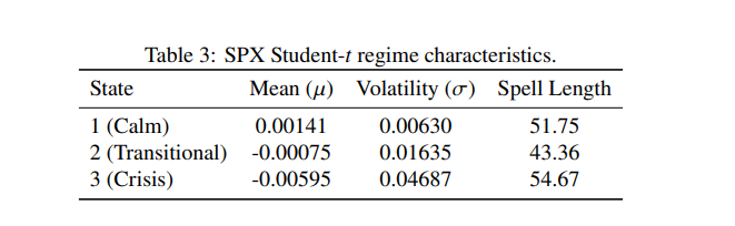
• Mathematical Signature: This state is defined by extreme volatility ( > 0.046), significant negative drift ( « 0), and high concentration of tail risk (q3 = 0.14450).

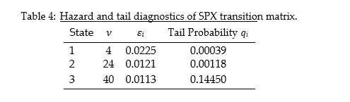
• Tail & Hazard Dynamics: Paradoxically, while this state represents maximum catastrophic intensity, it exhibits the highest degrees of freedom (v = 40) and the lowest hazard leakage (3 = 0.0113) in the SPX system. This indicates that the crisis is duration-driven: the system becomes trapped in a high-volatility basin where probability mass remains persistent rather than rapidly leaking out.

• Behavioral Context: Identified as a “2008 Liquidity Trap,” this regime is characterized by forced liquidations, repeated limit-down moves, and a collapse of the bid–ask spread.

• Fragility Status: Maximum. The system exhibits Catastrophe Fragility, where the probability mass is fully concentrated in the “Ruin Zone.”

State 2: Transitional/Steady (The “Escalation” Regime)

• Description: The Steady regime is the most deceptive state, appearing stable while underlying instability begins to accumulate.

• Mathematical Signature: Characterized by moderate volatility ( ≈ 0.016) and near-zero or slightly negative drift ( < 0).

• Tail & Hazard Dynamics: This state functions as a structural conduit with a tail probability (q2 = 0.00118) and moderate degrees of freedom (v = 24). The hazard leakage (2 = 0.0121) exceeds that of the Crisis state, indicating that structural integrity begins to degrade prior to full systemic rupture.

• Behavioral Context: Represents the “normalization” phase in which markets transition away from a tranquil bull regime but have not yet entered panic dynamics.

• Fragility Status: Increasing. As volatility expands, the probability mass begins to migrate toward the tails, increasing transition intensity (a23 = 0.0033) toward the Crisis state.

In the COR model (Figure 1), leakage via a23 represents the probability mass that exits the modeled system due to systemic rupture, liquidations, or structural failure. For each state i, the

leakage is defined by the row sum deficiency: _i = 1 − .3 A _{i j} . Hence, the value of a23 = 0.0033 is the critical gatekeeper for SPX. While the leakage (2) at this stage is almost zero, this transition intensity represents the flow of probability mass from a stable equilibrium into the Crisis state.

State 3: Calm (The “Stationary” Regime)

• Description: The Calm regime represents a high-entropy equilibrium state in which the market exhibits stable, mean-reverting dynamics.

• Mathematical Signature: Characterized by very low volatility ( ≈ 0.006) and positive drift ( > 0), consistent with a locally stable stochastic equilibrium.

• Tail & Hazard Dynamics: This regime exhibits tightly concentrated probability mass with negligible tail exposure. Hazard leakage remains minimal ( ≈ 0), indicating strong containment within the central region of the distribution and high structural integrity.

• Behavioral Context: Represents the “Goldilocks” environment, where liquidity is abundant and price dynamics are dominated by small, approximately Gaussian fluctuations.

• Fragility Status: Low. The system resides in a stable basin with minimal probability-mass dispersion, implying low transition pressure toward higher-risk regimes.

Hazard and Tail Risk Structure

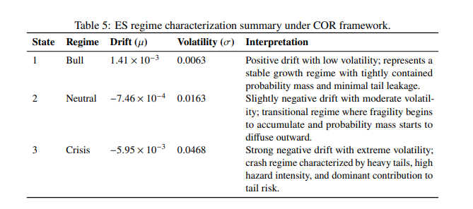
The crisis regime displays significantly elevated tail probability, indicating concentration of extreme downside risk (Table 4). State 1 (Bull) is characterized by the highest positive drift and lowest volatility, though the low degrees of freedom (v = 4) indicate significant fat-tailed risk even during growth periods. State 2 (Neutral) acts as a near-Gaussian state (v = 100) with moderate volatility and a slightly negative mean return. State 3 (Crisis) represents the depth of the 2008 financial crisis, exhibiting extreme volatility (0.030853) and the longest expected persistence of 132.14 days.

The COR model effectively aggregates these distinct states into a single, unified survival outlook for a 250-day trading horizon: the calculated Residence-Weighted Tail Probability (q¯) is 0.011956, which represents the average probability of a tail event occurring across the different regimes. This is complemented by a Residence-Weighted Hazard (^¯) of 0.014943, reflecting the integrated risk of leaking out of a stable state into a ruin event. Ultimately, for a horizon of T = 250, the model establishes a Ruin Bound of 0.043681, indicating approximately a 4.37% probability of the system failing to survive the specified threshold over the course of a trading year.

Findings for ES

Model Selection and Identification

This analysis provides a dissection of the Clock of Regimes (COR) analysis for the E-mini S&P 500 Futures (ES) during the 2007–2009 period. This model identifies the survival geometry of market regimes by treating transitions as a leaky system. The analysis compares two Hidden Markov Model (HMM) specifications to determine which best captures the statistical properties of the ES returns: The Student-t HMM log-likelihood (2155.14) is significantly higher than the Gaussian HMM (2148.76). This indicates that the ES price action during the financial crisis was characterized by heavy tails and extreme outliers that the Gaussian model fails to accommodate (Table 5).

Transition Dynamics

Gaussian Transition Matrix A : The Gaussian HMM identifies these transition probabilities:

Student- t Transition Matrix A : The Student-t model, which achieved a higher log-likelihood of 2155.14, identifies the following dynamics:

Both matrices demonstrate strong diagonal dominance (a_ii > 0.95), indicating that market regimes are highly persistent day-to-day. Both models show a 0.000000 probability for direct transitions between State 1 (Bull) and State 3 (Crisis), reinforcing that the COR model idiom that the system must transition through the neutral State 2. In the Student-t model, State 1 is more stable (0.9807) than in the Gaussian model (0.9581), which directly influences the exit rates calculated in the generator k.

Hazard-Adjusted Survival Operator

The Hazard-adjusted survival operator Q for the E-mini S&P 500 Futures (ES) represents the transition dynamics modified by the local survival probabilities of each regime. Based on the provided COR analysis report, the matrix is defined as follows,

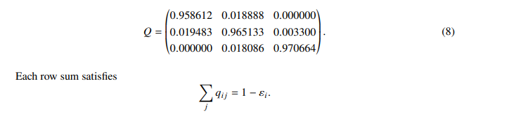
Similar to the SPX model, there is a 0.000000 probability of a direct jump between State 1 (Bull) and State 3 (Crisis), indicating the system must transition through State 2 (Adjacency Constraints). The rows sum to less than 1.0 (Sub-stochastic Property), where the missing probability mass represents the daily hazard or risk of entering a ruin state from that specific regime. State 3 (Crisis) shows the highest persistence in this operator at 0.970664, followed by State 2 (0.965133) and State 1 (0.958612).

The COR Generator Matrix

The COR generator k  matrix is derived from the hazard-adjusted transition operator Q as K = Q − I. This matrix represents the instantaneous flow rates between regimes and the local leakage (risk) or hazard rate of each system state.

The diagonal elements (Exit Rates) represent the total rate of exit from each state. State 1 has the highest exit rate at −0.041388, indicating it is the least stable regime in this survival geometry. The off-diagonal values (Flow Dynamics) indicate the specific rates of transitioning between states. For instance, the rate of moving from the Neutral State 2 to the Bull State 1 is 0.019483. Because the rows do not sum to zero, the missing probability mass (Hazard Content) represents the local hazard rate for each state. This contributes to the residence-weighted hazard (¯) of 0.015945.

The Fundamental Matrix

The Fundamental Matrix N = −K⁻¹ is the centerpiece of the COR model’s survival analysis. It translates the instantaneous flow rates of the generator K matrix into the expected number of days the system will reside in each state before leaking or Vfailing due to a tail event.

The diagonal elements N _iirepresent the total expected time spent in State i given the system started there. State 2 (Neutral) has the highest expected residence at 41.77 days, followed by State 3 (Crisis) at 36.98 days.

The off-diagonal elements show how much time probability mass in one state contributes to another (Inter-Regime Support) before exiting. For instance, if the system starts in the Crisis regime (State 3), it is only expected to spend 12.12 days in the safer Bull regime (State 1) before hitting the ruin threshold, reflecting the gravitational pull for probability mass of high-volatility states. Summing the rows of N gives the total expected time until a ruin event occurs (Total Expected Life) for each starting state. For a system starting in State 2, the total life expectancy is approximately

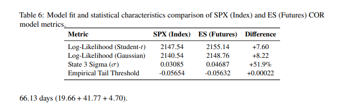
Quantitative COR model comparison of SPX and ES.

A quantitative comparison between the SPX (S&P 500 Index) and ES (E-mini S&P 500 Futures) COR analyses reveals that while both datasets identify three distinct regimes during the 2007–2009 crash period, the ES futures exhibit higher volatility and greater tail risk (Table 6). Both analyses found the Student-t HMM to be superior to the Gaussian HMM in terms of log-likelihood and AIC, confirming that asset returns during this period had significant fat tails.

Regime Residence and Stability: The Fundamental Matrix (N) highlights the expected number of days the system resides in each state before leaking or failing. The ES futures show shorter expected residence in the Neutral state (41.77 days) compared to the SPX (47.89 days). The SPX spent significantly more time in the High-Volatility Crisis regime, with a residence-weight of 20.61% , compared to only 12.25% for the ES futures. In the Generator Matrix (K ), the exit rate for the Bull state (State 1) is higher for SPX (−0.0433) than for ES (−0.0414), suggesting slightly less stability in the index’s growth regime during this window.

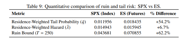
Risk and Ruin Analysis: The primary distinction between the two datasets lies in their integrated risk metrics over a 250-day horizon. The ES futures Tail Probability (q¯) exhibits a residence-weighted tail probability of 0.0184, which is 54% higher than the SPX’s 0.0119. The integrated hazard rate (^¯) for ES of 0.0159 exceeds that of the SPX at 0.0149. Finally, the probability of crossing the ruin bound’s threshold over the 250-day horizon is substantially higher for the ES futures market (7.08%) than for the SPX cash index (4.37%).

Comparison of State Summaries (Student- t): Table 7 provides a quantitative comparison of the Regime Means () and Expected Spell Durations (in days) between the S&P 500 Index (SPX) and the E-mini S&P 500 Futures (ES) during the 2007–2009 period. State 1 (Bull): Both assets show positive drift, with ES exhibiting a slightly higher mean return (1.41 × 10⁻³) and a longer expected

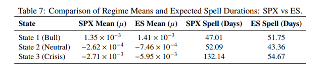
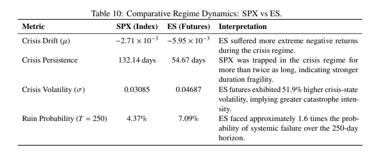
stay of 51.75 days compared to the SPX’s 47.01 days. State 2 (Neutral): This regime is characterized by a slight negative drift in both cases. The SPX remains in this state longer (52.09 days) than the ES futures (43.36 days). State 3 (Crisis): The most significant divergence occurs here. The ES futures experienced a much deeper negative drift (−5.95 × 10⁻³) than the SPX (−2.71 × 10⁻³). However, the SPX shows a far greater persistence in this regime, with an expected spell of 132.14 days compared to just 54.67 days for the ES.

Severity vs. Duration: While the ES futures suffered more extreme negative returns during the Crisis state (−5.95 × 10⁻³) compared to the SPX (−2.71 × 10⁻³), the SPX (cash index) tended to remain trapped in that regime for more than twice as long, with an expected spell of 132.14 days versus 54.67 days for the ES.

Market Sentiment: The Neutral state acts as a primary residence for the SPX, evidenced by an expected spell of 52.09 days, while the ES futures show more frequent movement between the Bull and Crisis extremes, reflected in shorter Neutral spells of 43.36 days.

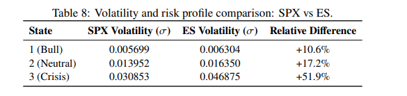
Risk Divergence: Table 8 presents a quantitative comparison of the volatility () and tail-risk parameters between the SPX (Index) and ES (Futures) datasets based on the Student-t HMM results. The most dramatic difference occurs in State 3, where the ES futures exhibit over 50% higher volatility than the underlying index. This suggests that during the height of the 2007–2009 crisis, the futures market absorbed significantly more variance and selling pressure than the cash index.

The SPX Bull regime (State 1) has a degree-of-freedom parameter v = 4 (tail heavyness), matching the ES Bull regime. This indicates that both markets possessed similar fat tails even during periods of growth. In the Crisis regime, the ES has a localized tail-event probability (q_tail) of 0.144499, which is more than 2.5 times higher than the SPX’s 0.057500 in the same state. Due to the higher volatility and local tail risk in the futures, the residence-weighted hazard (¯) for ES is 0.015945, compared to 0.014943 for the SPX.

Comparative Fundamental Matrices (N): The following provides a side-by-side comparison of the Fundamental Matrix (N = −K⁻¹) for the SPX and ES datasets to quantify the difference in total life expectancy and regime support during the 2007–2009 period. For the S&P 500 Index (SPX):

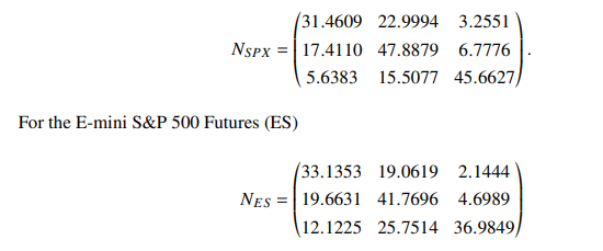
Summing the rows of N reveals the total expected days until a ruin event occurs. A system starting in the Neutral state (State 2) has a life expectancy of 72.08 days for the SPX compared to 66.13 days for the ES, indicating the futures market faced a 9% faster decay toward ruin. The diagonal elements show that the SPX remained in a Neutral state (State 2) for an average of 47.89 days, while the ES only managed 41.77 days. If the system starts in the Bull state (State 1), it is expected to spend 3.26 days in the Crisis state (State 3) for SPX, but only 2.14 days for ES. This suggests that while ES regimes are more volatile, the index (SPX) had a stronger gravitational pull into prolonged crisis residency. Starting from the Crisis state (State 3), the SPX is expected to spend only 5.64 days in the Bull state before ruin, whereas the ES expects 12.12 days. The futures market showed more bounce or mean-reversion potential, even if the moves themselves were more severe. Ruin Bounds: Table 9 presents a comparative analysis of the Ruin Bounds over a 250-day horizon (T = 250) highlighting the increased risk profile of the futures market relative to the cash index during the 2007–2009 period. The ES futures exhibit a significantly higher probability mass in the tails (q¯ = 0.0184) compared to the SPX index (q¯ = 0.0119). While the hazard rates (¯) are relatively close, the non-linear expansion of risk over the 250-day horizon results in a 7.09% ruin probability for the ES futures, nearly 1.6 times higher than the SPX’s 4.37%.

Despite both models using a similar empirical left-tail threshold (approximately −0.056), the higher volatility and frequency of extreme shifts in the ES data drive a much more aggressive ruin bound. Because the generator k matrix is an open/leaky operator, these ruin bounds are derived from the residence-weight vector implied by the Fundamental Matrix (N), providing a more realistic long-term risk assessment than static HMM averages.

Overview

This discussion examines the Clock of Regimes (COR) model, a structural framework for financial fragility that integrates regime-switching econometrics, survival analysis, and operator methods to quantify systemic risk and ruin probability. In this model, risk is no longer treated as a one-period variance statistic, but as a temporal survival problem. The central conceptual contribution of the COR model is to reinterpret regime switching as an open system in which probability mass does not merely move across latent states but can also leak out through regime-specific hazard channels. That change is decisive. In ordinary hidden Markov work, the focus is usually on filtered state classification, transition persistence, and perhaps volatility segmentation. In the COR framework, however, the object of interest becomes the survival-weighted geometry of the system: how long the probability mass remains concentrated in adverse states, how easily it escapes, and how the tail profile of each regime transforms local stress into cumulative ruin exposure. This operator-based shift from static probabilities to temporal exposure is what gives the COR framework its originality and explanatory power.

Theoretical Architecture and Operator Bridge

The COR model fundamentally reinterprets financial risk as a leaky dynamical system where systemic probability mass—defined as the content of probability accumulated over time—dissipates through regime-specific hazard rates. The model transitions through a hierarchical operator structure which is the backbone of the model: A → Q→ K → N.

The transition A matrix describes the discrete-time closed-system dynamics of the market. The open transition operator matrix (Q) adjusts the A matrix for leakage parameters (_i), reflecting the probability of systemic structural exit, such as liquidation or market shutdown. The COR generator K matrix represents the continuous-time instantaneous rates of flow and hazard between regimes. The Fundamental Matrix, N, is derived as N= −K⁻¹. This matrix calculates the expected residence or duration time (temporal exposure) the market spends in each regime before exiting the system.

The COR architecture allows for a Spectral Fragility Principle, where an increase in the spectral radius of the fundamental matrix, _P(N), indicates an expansion of survival-weighted residence time in adverse regimes, signaling growing systemic instability.

Empirical Findings: SPX vs. ES (2007–2009)

Empirical implementation using daily data from the Global Financial Crisis crash confirms that a Student-t  HMM specification is statistically superior to Gaussian alternatives. The Student-t model achieved significantly higher log-likelihoods for both the S&P 500 Index (2147.54) and E-mini S&P 500 Futures (2155.14), highlighting the necessity of capturing fat tails to evaluate catastrophe fragility. The study identified three distinct states: Stress/Crisis, Steady/Neutral, and Calm/Bull. Table ?? presents a quantitative comparison revealing divergent failure pathways for these structurally similar markets.

Fragility Decomposition and Ruin Bounds

The COR framework decomposes financial instability into two primary channels: (i) Duration Fragility, which arises when a system remains persistently trapped in unfavorable conditions (e.g., the SPX’s prolonged 132-day crisis spell), and (ii) Catastrophe Fragility, which reflects extreme tail losses that produce rapid destruction over short horizons (e.g., the high-intensity −5.95 × 10⁻³ drift in ES).

The model aggregates these factors into a Residence-Weighted Ruin Bound. Despite similar empirical left-tail thresholds (≈ −0.056), the ES futures market demonstrated a more aggressive ruin bound (0.070855) compared to the SPX index (0.043681). This disparity stems from the futures market’s higher residence-weighted tail probability (q¯ = 0.0184), which is 54% higher than the SPX index.

Discussion

The COR model provides a coherent and ambitious interpretation of financial fragility in which risk is no longer treated as a one-period variance statistic, but as a temporal survival problem. The Talebian view, as articulated by Nassim Nicholas Taleb Taleb (2016), is a philosophical and mathematical framework centered on how systems handle uncertainty, disorder, and Black Swan events ?. It rejects conventional Gaussian risk models in favor of a structural approach to fragility and ruin. The COR model closely aligns with the Talebian view by shifting the focus from thin-tailed, linear risk metrics to the nonlinear, temporal reality of systemic fragility. In this framework, risk is not a static one-period variance statistic like Standard Deviation or Value-at-Risk (VaR), but a survival-weighted accumulation of exposure to ruin.

At the theoretical level, the architecture A → Q →K→N is the backbone of the COR model. The closed-system transition matrix A describes ordinary regime switching, but it is deliberately treated as incomplete for real financial systems because actual markets are open to liquidation, structural breaks, funding collapses, and exit events that lie outside the state space. The hazard-adjusted operator Q corrects this by shrinking each row of A according to state-specific leakages_i. Once this is done, the generator-like matrix K = Q −I and the fundamental matrix

N = −K⁻¹ convert a discrete switching model into a continuous-time survival geometry. This is not a cosmetic reformulation. The entries of N measure expected survival-weighted residence time (duration), so the model can quantify not only whether a crisis regime exists, but how much temporal probability mass accumulates in it before the system exits. That move is especially important for markets, because many failures are not driven by single shocks alone but by prolonged exposure to unfavorable conditions.

This paper frames fragility through two distinct channels, and that decomposition is one of the strongest parts of the paper. Duration fragility refers to prolonged residence in adverse regimes. In practical terms, this is the case where a market does not necessarily crash instantaneously, but becomes trapped in a stressed condition long enough for cumulative damage to mount through deleveraging, liquidity withdrawal, credit contraction, or repeated losses. Catastrophe fragility, by contrast, refers to states whose tail distributions are so severe that large losses can materialize very quickly, even without long persistence. The importance of the COR model is that it can represent both mechanisms simultaneously. A system may be fragile because it remains too long in a moderately bad regime, or because it briefly touches a highly destructive tail regime, or because both effects reinforce one another. Standard risk models often blur these channels together. The COR model cleanly separates them. The Cor model demonstrated that while futures markets (ES) absorb more extreme catastrophe shocks, cash indices (SPX) may exhibit greater duration fragility through prolonged entrapment in high-volatility basins.

This paper highlights two major shortcomings in financial econometrics. The first issue is the reliance on Gaussian or diffusion-style assumptions, which often downplay extreme observations and treat volatility as too stable. The second concern revolves around the use of standard Hidden Markov Models (HMMs) with geometric residence-time structures, which can underestimate the clustering and persistence of crisis conditions. This critique is valid. In crisis data, it’s important to recognize that not only are returns fat-tailed, but time itself also becomes asymmetric. Stress episodes cannot be treated as interchangeable with calm episodes simply because they occupy the same time unit. A week during a crisis has a different economic significance compared to a week in a calm period. The COR model formalizes this concept by defining probability mass as temporally accumulated probability, rather than just an instantaneous measure.

That definition of probability mass is more than rhetorical. It clarifies why the fundamental matrix N is so central. In standard probabilistic language, one asks for the probability of being in state i at time t. In the COR framework, one also asks how much total time-weighted probability is expected to reside in each state before structural exit. This gives a more natural metric for fragility in environments where repeated or prolonged exposure matters. A market that spends modest probability in a crisis state for a very long time may be more dangerous than a market that touches a more extreme regime only briefly. The model therefore replaces static regime identification with temporal geometry.

The open transition operator Q is especially important because it formalizes the notion that regime switching alone is not the whole story; the system is also subject to survival loss. In economic terms, the hazard vector acts like a structural permeability parameter. Higher hazard means the regime is less capable of containing probability mass and more likely to transmit it into systemic failure, absorption, or external ruin. This is why the rows of Q sum to less than one. The missing probability mass is not numerical error. It is the model’s explicit representation of openness.

The generator identification result is also conceptually useful because it places the model within a broader continuous-time tradition. Even if the empirical estimation begins with a discrete HMM, the transition to K and N gives access to tools familiar from compartmental analysis, survival theory, and continuous-time Markov processes. That is a strong interdisciplinary move. It allows the paper to speak not only to financial econometrics but also to mathematical systems theory. The operator bridge theorem makes that explicit: the model progressively translates persistence into hazard-adjusted survival, then into generator form, and finally into residence-time (duration) structure. Each step changes the interpretation of the same underlying market process without discarding information.

The fragility decomposition theorem is one of the clearest summaries of the model’s intuition. Fragility is treated as the interaction of residence mass, tail severity, and hazard leakage. This multiplicative logic is economically sensible. Residence mass captures temporal exposure. Tail severity captures the intensity of adverse outcomes conditional on being in a state. Hazard leakage captures the openness of the system and thus its vulnerability to structural loss. None of these alone is sufficient. A regime can have heavy tails but low residence mass, or long residence but mild tails, or high hazard but little persistence. True systemic fragility emerges when all three are sufficiently active together. That formulation is one of the paper’s most useful contributions because it explains why similar markets can fail differently.

The spectral fragility principle extends the framework beyond simple summary metrics. By linking fragility to the spectral radius of N, the paper proposes an operator-level early-warning concept. A larger _P( N) means an expansion of survival-weighted residence time, which in turn means that adverse structures are becoming more persistent or more difficult to escape. This is appealing because it makes fragility a property of the whole system, not just a property of one regime parameter. Spectral diagnostics are particularly attractive in crisis analysis because they may move before realized collapse occurs. In that sense, the COR model is not merely descriptive; it has potential as a monitoring device.

Using Student-t emissions for the latent regimes is essential. Heavy-tailed distributions are not optional in crisis-era data, and the use of regime-specific degrees of freedom vi allows the tail profile itself to vary across market states. This is important because calm, transitional, and crisis conditions do not differ only in mean and volatility; they may differ in the shape of their tails. The hazard calibration_i=_min + cl_vi is elegant because it ties system openness directly to tail thickness. Regimes with smaller vi are more heavy-tailed and therefore more structurally leaky. That mapping gives the model a tight internal logic: tail behavior influences hazard, hazard influences Q,Q influences K, and K determines the temporal geometry through N . The results for SPX strongly support the paper’s theoretical claims. First, the Student-t HMM outperforms the Gaussian model in log-likelihood and AIC, which confirms that heavy tails matter materially for the 2007–2009 period. This is a crucial empirical validation of the model’s premise. The gain in fit is not merely statistical housekeeping; it indicates that crisis returns cannot be adequately described by thin-tailed within-regime shocks. The paper rightly interprets this as evidence that catastrophe fragility is an intrinsic feature of the data.

Second, the transition matrices reveal a highly persistent three-state regime structure. All diagonal elements exceed 0.95, so the system is sticky in every state. That alone would already be important, but the absence of direct transitions between the calm and crisis states is even more informative. It means that the market generally moves through an intermediate regime rather than jumping directly from tranquility to rupture. This supports the interpretation of the middle state as a conduit of fragility accumulation. In COR model terms, the system is path-dependent: deterioration tends to occur through an escalation channel rather than through instantaneous discontinuity.

The hazard-adjusted operator Q deepens that interpretation. Because its rows sum to less than one, the market is explicitly modeled as a leaky survival system. The missing row mass is the local hazard content, which makes the state process economically richer than a standard Markov chain. The generator K then shows which states are more transient and which flows are more relevant. In the SPX case, the bull state has the highest exit rate, suggesting that calm growth is relatively easy to leave during the crisis sample. That is a telling result: the safe regime is structurally fragile, even if its one-step volatility is low.

S&P 500 Index (SPX)

The SPX fundamental matrix is especially revealing. Its diagonal entries indicate substantial residence in all three states, but particularly in the transitional and crisis states. The interpretation is powerful: the market during 2007–2009 was not merely volatile; it was trapped. This is the empirical manifestation of duration fragility. The system did not only experience bad states; it accumulated time within them. Off-diagonal entries add further nuance by showing how one state supports residence in another before exit. The neutral state, in particular, appears to function as the main staging area through which adverse persistence is transmitted.

The SPX state summary illustrates the economic meaning of the latent regimes. The bull state combines positive drift with low volatility, but still has heavy tails. This is important because it shows that apparently favorable conditions are not free of fragility. The neutral state is close to Gaussian and serves as the dominant transitional basin. The crisis state combines high volatility, negative drift, and long expected spell duration, which makes it the natural locus of duration fragility. The very long expected spell in the crisis state is a critical empirical finding. It says that during the financial crisis, systemic stress in the cash index was not only severe; it was persistent enough to become structurally entrapping. The SPX hazard and tail diagnostics reinforce this picture. The crisis state has by far the largest tail probability, so catastrophe risk is concentrated there. Yet the hazard structure also matters. The interplay between v,_i, and q_i shows that the most dangerous state is not simply the one with the worst volatility reading, but the one where heavy tails, persistence, and leakage jointly support ruin accumulation. That is precisely the advantage of the COR model framework: it converts descriptive regime labels into a measurable structural mechanism.

The aggregate SPX measures summarize this mechanism cleanly. The residence-weighted tail probability q¯ = 0.011956, the residence-weighted hazard ^¯ = 0.014943, and the one-year ruin bound of 0.043681 provide a compact survival-based view of systemic risk. Their interpretation should be handled carefully. These are not plain unconditional probabilities in the usual sense; they are structural summaries induced by open-system survival dynamics. The ruin bound, in particular, is best understood as an upper-bound style measure of systemic vulnerability over the horizon, not as a literal point forecast of collapse. Even so, a value around 4.37% is substantial for a broad market index and confirms that the 2007–2009 period involved a nontrivial structural probability of severe degradation..

E-mini S&P 500 Futures (ES)

The ES results are equally important, and perhaps even more informative from a comparative perspective. Again the Student-t model beats the Gaussian specification, with an even larger log-likelihood. This confirms that futures returns are even more strongly shaped by heavy tails and outliers. That fits the economic intuition that the ES, because of leverage, round-the-clock trading, and liquidity concentration, should absorb stress more violently than the underlying cash index. The paper correctly interprets this as evidence that the futures market is structurally more exposed to explosive tail dynamics.

The ES regime characterization makes that clear. The bull state is similar to SPX in sign and scale, but the neutral state is more negative and the crisis state is dramatically more severe. The crisis-state volatility is much larger than in SPX, and the negative drift is considerably deeper. This suggests that when the futures market enters the crisis regime, it experiences a sharper catastrophe channel. In other words, ES appears more catastrophe-fragile than SPX. The market does not merely become volatile; it becomes violently nonlinear.

Yet the transition and residence results show that ES is not simply worse in every dimension. Its crisis-state spell duration is much shorter than SPX’s, and its fundamental matrix indicates less prolonged residence in crisis. This is where the paper’s decomposition becomes very useful. ES is more severe but less durationally trapped. SPX is less severe but more durationally trapped. Thus the two markets fail through different fragility pathways. ES expresses catastrophe fragility more strongly; SPX expresses duration fragility more strongly. That is one of the most valuable empirical conclusions in this paper.

The comparative tables support this reading well. The higher State 3 volatility in ES, the similar empirical tail threshold, and the much larger residence-weighted tail probability all indicate that futures carry much stronger extreme-risk intensity. At the same time, the much longer SPX crisis spell shows that the index absorbs stress through persistence and prolonged malaise. This is an important distinction for practitioners. A leveraged or derivative market may destroy wealth faster, while the cash benchmark may trap capital for longer. Both are fragile, but in different ways.

The comparative fundamental matrices deepen the interpretation. ES has shorter total expected life starting from the neutral state, which suggests faster decay toward ruin. But ES also shows more ability to spend some time in the bull state even after starting in crisis, implying more bounce or snapback potential. That too is economically plausible. Futures markets are often more violent in both directions: they can crash faster but also rebound faster. SPX, by contrast, appears to retain a stronger gravitational pull into prolonged crisis residency. This is a beautiful illustration of how the same broad market ecosystem can contain two distinct temporal architectures of risk.

The comparative ruin metrics bring the whole argument together. ES has a residence-weighted tail probability more than 54% higher than SPX, a slightly higher residence-weighted hazard, and a ruin bound over 62% higher. The modest difference in hazard but large difference in ruin bound is especially interesting. It implies that nonlinear amplification is being driven primarily through the tail channel rather than through much larger openness per se. In other words, the futures market is not vastly more fragile because it leaks much more often, but because when it is stressed, the consequences are far more severe (catastrophe-fragility).

Conclusions

There is also a deeper conceptual strength of the COR model worth emphasizing. The paper does not treat hazard as exogenous noise added after regime estimation. Instead, hazard is integrated into the regime architecture itself through the open-system formulation. This makes the model much more than an HMM with a tail overlay. It becomes a structural theory of how persistence, tail thickness, and openness interact. That operator-theoretic viewpoint is what allows the paper to link econometrics with survival analysis and compartmental methods in a nontrivial way.

From a systemic-risk perspective, the key message is that fragility cannot be read off volatility alone. A low-volatility state may still be heavy-tailed. A moderate-volatility state may become the main conduit of fragility accumulation. A crisis state may matter either because it is so destructive or because it is so persistent. The COR model forces these distinctions into the open. This is a major conceptual improvement over one-factor risk summaries or unconditional tail measures.

The spectral component also opens the door to future work. If rolling estimation is implemented, changes in p( n), residence weights, and hazard-adjusted eigenstructure could provide forward-looking indicators of instability before realized market collapse. That would move the model from retrospective diagnosis to active surveillance. Given the paper’s emphasis on early-warning construction, this is one of the most promising empirical extensions.

The COR model presents a strong and original framework. The COR model contributes a mathematically disciplined way to think about systemic fragility as temporal content of adverse probability mass under open dynamics. The empirical comparison between SPX and ES is especially compelling because it demonstrates that two closely related markets can embody different failure geometries: the cash index more duration-fragile, the futures contract more catastrophe-fragile. That distinction is exactly the kind of structural insight standard volatility or HMM summaries often miss. In that sense, the paper succeeds in showing that survival-weighted exposure, rather than variance alone, is the right language for ruin-sensitive financial analysis.

The COR model provides a unified framework for quantifying ruin exposure by shifting risk assessment from static probabilities to temporal geometries of probability mass. By integrating hazard-induced openness, the model demonstrates that while futures markets (ES) absorb more extreme catastrophe shocks, cash indices (SPX) may exhibit greater duration fragility through prolonged entrapment in high-volatility basins.

Acknowledgments

Mathematics were manually audited by the authors, verified for mathematical accuracy using Wolfram Mathematica 14.3, and refined to ensure alignment with the theoretical model.

Funding

This research did not receive any specific grant from funding agencies in the public, commercial, or not-for-profit sectors.

Mathematical Appendix

A Open Transition Operator

Theorem A.1 (Hazard-Adjusted Transition Operator). Let A be a k × k stochastic transition matrix representing a closed regime system, where 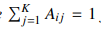    Define the hazard-adjusted transition operator Q as:

                                                              
where 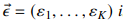  is a regime-dependent hazard vector with 0 ≤ _i ≤ 1 for each i. Then, Q is a substochastic matrix such that each row sum satisfies:

                                                                

This construction transforms the regime-switching process into an open Markov system, where the evolution of the system tracks survival-weighted probability mass and accounts for potential absorption outside the modeled regime system.

Proof. The proof that the hazard-adjusted transition operator Q is a substochastic matrix proceeds as follows:

1.Properties of the Stochastic Matrix A: By definition, the transition matrix A is a stochastic matrix representing a closed regime system. All  A _ij entries c are non-negative, and each row i sums to unity:

                                                      
2. Definition of Q : The operator Q is defined by scaling the rows of A by a regime-dependent hazard vector →:

                                                   

where each leakage parameter satisfies 0 ≤ _i ≤ 1. Consequently, each entry Q_ij = (1 −_i) A _ij  .'

3. Row Summation of Q : Consider the sum of the entries in the i -th row of Q :

                                                       

Substituting the stochastic property _.j A _ij  = 1, we obtain:

                                               

4. Substochastic Property: Given the constraint 0 ≤ _i ≤ 1, it follows that 0 ≤ 1 − _i ≤ 1. Therefore, the row sum of Q is bounded:

                                            
5. Conclusion: The matrix Q  is substochastic because all its entries are non-negative and the sum of each row is less than or equal to 1. This reduction by _i represents probability mass leaving the system, reflecting the possibility of absorption outside the modeled regime system. Thus, Q  describes an open Markov system tracking survival-weighted probability mass.

                                               

Theorem A.2 (Generator Proxy Identification). Let Q  be the hazard-adjusted transition operator of a discrete-time regime system, and let I be the identity matrix. Define the generator matrix K  as:

For a small time step Δt, the matrix K serves as a discrete-time approximation of the continuous-time Markov generator. This construction establishes an operator bridge linking discrete Hidden Markov Models (HMMs) to continuous-time survival processes via the fundamental relation N = −K^−1.

Proof. The role of the generator matrix K as a bridge between discrete Hidden Markov Models and continuous-time survival processes is established as follows:

1. Continuous-Time Dynamics: In a continuous-time Markov process, the transition probability matrix over an interval t is defined by the matrix exponential:

                                                        

For sufficiently small t , the first-order Taylor expansion provides the linear approximation:

                                                 

2. Discrete-Time Approximation: For a discrete-time step Δt, the transition matrix P of a Hidden Markov Model can be approximated using the rate matrix Q :

                                              

Substituting the definition of the COR generator K = Q −I (or Q = K +I) into the approximation yields:

                                                  

This confirms that the structure of K dictates the infinitesimal flow of the system[cite: 1, 2].

3. Connection to HMMs: The generator K approximates the behavior of a continuous-time process within a discrete framework. This allows Hidden Markov Models to represent underlying continuous-time dynamics, facilitating the analysis of market processes that transition over potentially infinitesimal time intervals.

4. Conclusion: The matrix K , derived from the hazard-adjusted operator Q , acts as a functional bridge between discrete and continuous-time models. It provides a rigorous pathway to analyze continuous-time survival processes—such as regime-specific residence times and ruin probabilities—through the lens of discrete-time HMMs.

This completes the proof that K serves as the infinitesimal generator proxy for the open regime system.

Theorem A.3 (Fundamental Matrix and Survival Geometry). The fundamental matrix of the open system is defined by the operator:

                                                        

The element N_ij represents the expected survival-weighted time spent in regime j when starting from regime i . Thus,N  provides a direct measure of temporal probability content.

In financial terms, large diagonal entries of N indicate durational entrapment in adverse regimes, while large off-diagonal entries reveal conduit states through which systemic fragility propagates. The fundamental matrix N = −K ⁻¹ may be derived by inverting the negative of the K matrix. The inverse of this matrix calculates the expected persistence of probability mass (residence time) within each node—essentially, the total time the market spends in a specific regime before it eventually leaks out or transitions.

Proof. To establish the equivalence , we proceed through the properties of the matrix exponential and its convergence requirements:

1. Matrix Exponential Definition: The matrix exponential e^kt is defined via the power series expansion, analogous to the scalar case:

                                         

where I denotes the K × K identity matrix.

2. Integration of the Matrix Exponential: Consider the improper integral of the matrix exponential from 0 to ∞:

                                                   

3.Term-by-Term Integration and Convergence: Integrating the series term-by-term, we observe:

                                                         

These terms appear to diverge unless the matrix k is negative definite or stabilizing (i.e., all eigenvalues have negative real parts). In the COR model, K = Q − I is an open/leaky generator proxy, ensuring that the eigenvalues of k are strictly negative, which guarantees the decay of e^kt as t → ∞.

4. Convergence and Inversion: Under the condition that K is invertible and its eigenvalues have negative real parts, we use the fundamental theorem of calculus for matrices:

                                                         

Integrating both sides from 0 to ∞:

                                                  

Since lim _t→∞ e^kt = 0 (due to negative eigenvalues) and e^k(0) = I:

                                                   
5. Conclusion: Premultiplying by k⁻¹, we obtain:

                                                  

The result N = −K⁻¹ is well-defined and holds provided K is transient, reflecting the expected persistence of probability mass within the regime system before structural exit or ruin.

Theorem A.4 (Fragility Decomposition). In a financial market characterized by K regimes, let qi denote the left-tail probability of returns conditional on regime i , _i denote the hazard leakage for regime i  andbe the survival-weighted probability of regime i such that 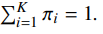The systemic risk measures are decomposed as follows:

1. Residence-weighted tail exposure (q¯):

2. Average hazard leakage (^¯)  :                               

This decomposition illustrates that financial markets exhibit fragility through two primary channels: duration fragility, where the system remains for extended periods in adverse regimes (_i),and catastrophe fragility, where losses mount rapidly during crisis episodes (q_i). These weighted sums provide a structural measure of how individual regimes contribute to systemic risk, linking heavy-tailed shocks and regime persistence to the operator-level survival geometry.

Proof. The derivation of the residence-weighted tail exposure (q¯) and the average hazard leakage (^¯) as systemic risk measures relies on the properties of weighted expectations over the survival-weighted regime distribution .

1. Derivation of Residence-Weighted Tail Exposure (q¯): By definition, the systemic tail exposure is the expectation of the regime-specific tail probabilities q_i over the long-run allocation of probability mass. Given that is the survival-weighted distribution derived from the fundamental matrix N , such that:

                                             

The aggregate measure q¯ is constructed as the convex combination:

                                            

This weighted average represents the expected probability of a tail event occurring at any given time, accounting for the varying durations the system spends in each latent state.

2. Derivation of Average Hazard Leakage (^¯): Similarly, let _i represent the instantaneous hazard leakage (or "openness") of regime i . The systemic hazard rate ¯ is the ensemble average of these local leakages across the survival geometry:

Sincereflects the expected residence time in each node, ^¯ quantifies the integrated rate at which probability mass exits the modeled system (ruin intensity).

Conclusion: Both q¯ and^¯ are valid structural descriptors of the open Markov system. They facilitate the mapping of discrete regime dynamics into a unified survival-oriented risk bound, _P(ruin) ≤ 1 − e−Th Λ, where Λ is a function of these residence-weighted averages.

Theorem A.5 (Spectral Radius and Norm Bound). Let A´ ∈ C^nxn be a square matrix, and let P( A)

denote its spectral radius, defined as the maximum absolute value of its eigenvalues:

                             
For any consistent matrix norm the spectral radius is bounded by the norm of the matrix:

                              
This property ensures that the spectral radius provides a lower bound for all matrix norms and is a critical measure for analyzing the stability, convergence, and structural behavior of linear operators in open dynamical systems.

Proof. To prove that the spectral radius p(A) of a square matrix A ∈ C ^n×n is bounded by any consistent matrix norm we proceed as follows:

1. Eigenvalue and Eigenvector Relationship: Letbe any eigenvalue of the matrix A, and let v be its corresponding non-zero eigenvector (v ≠ 0). By the definition of the eigenvalue problem, we have:

            

2. Applying the Matrix Norm: Taking the norm of both sides of the equation and utilizing the property of absolute homogeneity  we obtain:

                                

3. Consistency of the Matrix Norm: By the definition of a consistent matrix norm (submul-tiplicativity with respect to a vector norm), the following inequality holds for any vector v:

                         

4. Combining the Inequalities: Substituting the expression from Step 2 into the inequality from Step 3, we have:

                                      

Since is an eigenvector, v ≠ 0. Dividing both sides byyields:

                                         

5. Conclusion for the Spectral Radius: Since the inequality || ≤ holds for every eigenvalue ∈ (A), it must also hold for the maximum absolute value of those eigenvalues.

Therefore:

                                      

This completes the proof that the spectral radius of a matrix is bounded above by any consistent matrix norm.

Theorem A.6 (Residence-Weighted Ruin Probability Bound). Let T_h denote the risk horizon (e.g.,T_h = 250 days), and let q be the vector of regime-specific tail-loss probabilities. Given the survival-weighted regime distribution and the fundamental matrix N = −K⁻¹, the structural ruin probability for the open dynamical system is bounded by:

                                               

where 1 is the K × 1 summation vector. This bound captures the non-linear interaction between regime duration, tail exposure, and the systemic hazard structure.

Proof. To provide a rigorous derivation of the residence-weighted ruin probability bound, we integrate elements of stochastic processes, survival analysis, and operator theory. The proof is structured as follows: 1. Definition of Parameters: Let T_h denote the risk horizon. We define the following vectors and operators:

• : The survival-weighted regime distribution (weights).

• N :The fundamental matrix (N = −K⁻¹) capturing expected residence times.

• q : The hazard vector of regime-specific tail-exposure rates.

• 1: A K × 1 summation vector of ones.

2. System Dynamics and Survival: We model the regime switching as an open Markov process. Let S(t) be the survival function, representing the probability that the system has not encountered a ruin event by time t. The instantaneous transitions and “leakage” are governed by the generator K where N represents the integrated path of the system until exit.

3. Derivation of the Cumulative Hazard: The cumulative hazard over the horizon T_h is determined by the temporal content of probability mass residing in adverse states. In the COR framework, this is expressed as the product of the residence distribution and the tail-exposure rates:

                                         

Under the assumption of stationary regime dynamics within the horizon, the survival probability follows an exponential decay:

                                              

4. Establishing the Normalized Bound: To quantify the effective ruin intensity, we normalize the catastrophe volume (^T N _q) by the total expected system life expectancy (^T N1). This ratio defines the residence-weighted hazard rate Λ:

                                                
Integrating this rate over the horizon T_h, the probability of ruin is defined as the complement of the survival function:

Conclusion: The resulting bound captures the systemic interaction between regime duration (persistence), tail exposure (severity), and hazard structure (openness). The exponential term reflects the non-linear accumulation of risk, providing a robust measure of ruin probability in a non-ergodic environment.

Theorem A.7 (Tail-Sensitive Hazard Calibration). Let _i denote the hazard rate for regime i . For a given baseline structural openness min > 0 and a sensitivity constant c > 0, the hazard rate is calibrated as:

                                                  

where v_i represents the degrees of freedom (tail thickness) of the Student-t distribution associated with regime i . It follows that _i increases as v_i decreases, indicating that regimes with heavier tails (smaller v_i ) exhibit higher systemic leakage risk.

Proof. The proof of the tail-sensitive mapping proceeds by analyzing the functional behavior of the calibration equation:

1. Baseline Openness: The condition  min > 0 ensures that the system remains an open dynamical system (substochastic) even in the limit of infinitely thin tails (v_i→ ∞).

2. Sensitivity Control: The constant c > 0 acts as a scaling factor that adjusts how aggressively the hazard rate responds to changes in tail thickness.

3. Tail Thickness Analysis: In a Student-t distribution, the parameter v_i inversely correlates with tail heaviness; as v_i → ∞, the distribution approaches Gaussian, while small v_i values indicate extreme kurtosis and fat tails.

4. Monotonicity: Taking the partial derivative of _i with respect to v_i :

                                

Since c > 0 and  > 0, the derivative is strictly negative                                        

Conclusion: As v_i decreases (tails become heavier), the term increases, leading to a higher hazard rate _i. This formalizes the requirement that regimes characterized by extreme tail risk must exhibit higher systemic “leakage” or probability of ruin.

Theorem A.8 (Tail Risk Measurement Using Student-t Distribution). Let x_t be a random variable representing asset returns at time t and let s_t∈ {1, . . . , k } denote the latent market regime. Assume that for each regime i , the returns follow a Student-t  distribution with location _i, scale _i and degrees of freedom v_i.

1. Regime-Specific Left-Tail Probability: For a given significance level and a corresponding empirical threshold x_a the left-tail probability q_i for regime i is:

                                   

2. Aggregate Tail Exposure (q¯): The aggregate systemic tail exposure is the residence-weighted average of the local tail probabilities:

                                            

where _i is the survival-weighted probability (residence weight) of regime i derived from the fundamental matrix N

Proof. The measurement of aggregate tail risk follows from the conditional distribution properties of the Hidden Markov Model:

1. Computation of q_i : For each regime i the probability mass residing below the threshold x_a is calculated using the Cumulative Distribution Function (CDF) of the fitted Student-t

distribution:

                                    

This integral captures the heavy-tailed shocks unique to the volatility and kurtosis signatures of regime i .

2. Integration of Systemic Exposure: The aggregate exposure q¯ is the expected value of the indicator function I ( X_t ≤ x_a) over the survival-weighted state space. By the law of total probability applied to the residence distribution :

                                                   
Substituting the Student-t CDF for q_i completes the proof.                           

Theorem A.9 (Structural Ruin Metrics). The survival-weighted systemic risk of an open regime system is quantified by the following metrics:

1.Average Hazard Leakage (^¯): The integrated rate of probability mass dissipation across the survival geometry is computed as:

                                                  

where_i is the residence weight and _i is the regime-specific hazard rate.

2. Structural Ruin Probability Bound: Given a risk horizon T_h the probability of the system crossing a ruin threshold is bounded by:

                                     
This metric integrates regime persistence (via the fundamental matrix N), tail severity (via the hazard vector q ), and systemic openness (via and ) into a unified, survival-oriented risk measure. It formalizes the Talebian view of risk as a temporal survival problem rather than a static variance statistic.

B Proof of Generator Identification

Theorem B.1 (Generator Identification). Let AΔt denote the transition matrix of a regime system observed at time step Δt. Suppose there exists a matrix G such that

Then

      

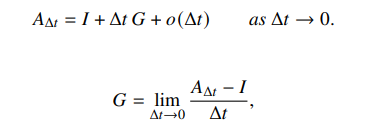
and G is the continuous-time generator of the limiting regime process.

Proof. By assumption,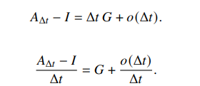

Dividing both sides by Δt gives

Since o (Δt)/Δt → 0 as Δt → 0, we obtain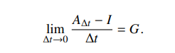

To verify that G is a valid continuous-time generator, note that eachis row-stochastic, so its rows sum to one. Hence

                                                                               
Substituting the expansion yields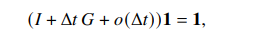                          

so                                                                        

Dividing by Δt and taking limits gives

                                                                                                G1=0

Thus the row sums of G vanish, as required of a continuous-time Markov generator. The off-diagonal nonnegativity follows from the fact that transition probabilities are nonnegative for sufficiently small Δt. Therefore G is the infinitesimal generator. 

C Proof of the Operator Bridge

Theorem C.1 (Operator Bridge). The sequence

                                                                        

defines a hierarchy of operators linking closed regime persistence to open-system temporal exposure. In particular:

1. A governs closed-state transitions;

2. Q governs survival-adjusted transitions;

3. K = Q − I governs the corresponding open-system generator dynamics;

4. N= −K⁻¹ = (I− Q)⁻¹ governs expected survival-weighted residence times.

Proof. The first two steps are definitional. Given a closed transition matrix A premultiplication by diag(1 − _i) reduces each row by the associated survival factor, yielding the substochastic operator Q Thus Q encodes one-step transitions conditional on non-exit.

Next, define                                                              K = Q -1.

 Then                                                                     -K = Q -1.

Because _P(Q) < 1, the matrix I− Q is invertible, and hence so is −K. Therefore

                                                               

Since _P(Q) < 1, the Neumann series converges: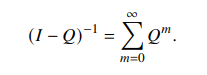       

 Thus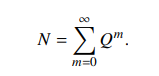                                                                                                                                                        

The (i, j) entry ofQ_m is the probability mass that, starting from state i, survives and occupies state j after m steps. Summing over m yields the expected total survival-weighted time spent in state j when starting from i. Hence N is the fundamental residence-time operator.

D Integral Representation of the Fundamental Matrix

Proposition D.1. If all eigenvalues of K have strictly negative real parts, then

                                                            

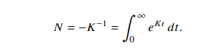
Proof. Consider the matrix-valued function e^Kt. Since the eigenvalues of K  have negative real parts, e^Kt → 0 as t → ∞. Also

                                                                           

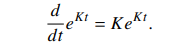
Integrating from 0 to T,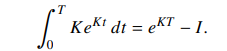                                 

Premultiplying by K⁻¹   ,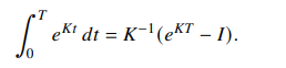                                           

Taking T → ∞, and using e^Kt → 0,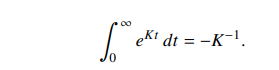

This is exactly N .

E Proof of the Fragility Decomposition

Theorem E.1 (Fragility Decomposition). Letbe a survival-weighted regime distribution, q = (q₁, . . . , q_k )^Tbe the vector of regime-specific left-tail probabilities, and let be the hazard vector. Define

                                                          

Let F_dur be any positive scalar functional of the residence structure, for example

                                                              

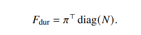
Then the composite index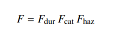                          

is increasing in each component and therefore furnishes a multiplicative decomposition of structural fragility into residence, catastrophe, and hazard channels.

Proof. Assume all three components are strictly positive. Then

                                                              
The partial derivatives are

                                                                

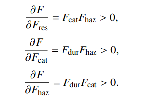
Hence F is strictly increasing in each argument. Therefore an increase in residence mass, catastrophe severity, or hazard leakage increases total fragility.

F Spectral Fragility Principle

Theorem F.1 (Spectral Fragility Principle). Suppose Q( is a family of substochastic matrices depending smoothly on a scalar parameter with _P (Q()) < 1 for all admissible Let

                                                             

If Q() increases entrywise in then N () increases entrywise in , and in particular P N ()) is nondecreasing in .

Proof. BecauseP(Q()) < 1, we have the convergent Neumann expansion

                                                                
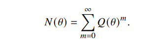
If Q () increases entrywise in, then for every positive integer m the matrix power Q () m also increases entrywise in, since matrix multiplication preserves order for nonnegative matrices. Hence each term in the series is nondecreasing entrywise, and therefore the sum N () is nondecreasing entrywise. Now N () is nonnegative. By Perron–Frobenius theory, the spectral radius of a nonnegative matrix is monotone with respect to entrywise order. Therefore _P(N ()) is nondecreasing in.

G Residence-Weighted Ruin Bound

Theorem G.1 (Residence-Weighted Ruin Bound). Let q = (q¹, . . . , qK )^T be the vector of regime-specific tail-loss probabilities, let be a survival-weighted regime distribution, and let N be the fundamental matrix. Define the effective ruin intensity

                                                                         
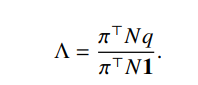
Then over a horizon T_h > 0, a structural ruin bound is given by

                                                                      

Proof. Interpret Λ as the average tail-event intensity under residence weighting. The numerator ^T N _q aggregates regime-specific tail probabilities weighted by expected survival-adjusted time spent in each state, while the denominator ^T N 1 normalizes by total expected residence time. Thus Λ is an average rate of ruin-relevant exposure.

If ruin events are dominated by a hazard process with effective rate at most Λ, then the survival probability over horizonT_h is bounded below by the exponential survival law,

                                                            

Therefore,                                             

This yields the stated bound.

H Existence of the Fundamental Matrix

Proposition H.1. If Q is substochastic and transient, then I− Q is invertible and

                                                                  

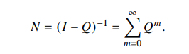
Proof. Transience implies _P(Q) < 1. By a standard result in matrix analysis, if the spectral radius of Q is strictly less than one, then the Neumann series converges absolutely:

                                                                                

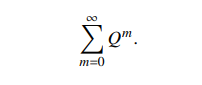
Moreover,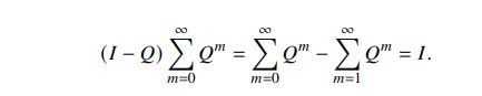                                  

Similarly,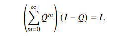                                             

Hence (I − Q)⁻¹ exists and equals the convergent series.

I Interpretive Corollary: Duration versus Catastrophe Fragility

Corollary I.1. Two systems may have different total fragility rankings depending on whether the ranking criterion emphasizes residence structure or tail severity. In particular:

1. a system with larger F_dur but smaller F_cat is more duration-fragile;

2. a system with smaller F_dur but larger F_cat is more catastrophe-fragile.

Proof. This follows immediately from the multiplicative decomposition

                                           

Holding F_haz fixed, the ranking depends on the relative sizes of the residence and catastrophe components. A system can dominate on one margin and be dominated on another. Hence fragility is not one-dimensional.

J Remarks on Identification and Empirical Implementation

The appendix results are intentionally abstract. In empirical implementation, the matrices A, Q, K, and N are estimated objects, and the regime-specific tail probabilities q_i  depend on the fitted emission law. The proofs above establish structural validity of the operator framework independently of the particular estimation scheme, provided that the estimated open system remains transient.

Remark J.1. The generator K = Q − I used in the main text is a discrete-time generator proxy. In applications with explicit time-step scaling Δt, one may use

                                                            

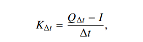
in which case all integral and inverse formulas carry over with the appropriate scaling.

Remark J.2. The spectral results do not require reversibility. They rely only on positivity and transience of the open system, together with Perron–Frobenius order properties for nonnegative matrices.

References

Foot notes

¹We define probability mass as the content of probability accumulated over an amount of time. In our COR architecture, probability is not treated purely as an instantaneous quantity p (x). Instead, it is temporally embedded. It reflects how much probability resides in a state across time.

References

- L. E. Baum, T. Petrie, G. Soules, and N. Weiss. A maximization technique occurring in the statistical analysis of probabilistic functions of markov chains. The Annals of Mathematical Statistics, 41 (1):164–171, 1970
- M. Berman and R. Shoenfeld. Invariants in experimental data on linear kinetics and the formulation of models. Journal of Applied Physics, 27:1361–1370, 1956.
- Cboe Exchange. Trade around the clock with cboe global trading hours. https://www.cboe. com/insights/posts/cboe-global-trading-hours/, 2026. Accessed: 2026-03-25.
- CME Group Inc. E-mini S&P 500 futures anoptions.https://www.cmegroup.com/markets/ equities/sp/e-mini-sandp500.html,2026. Accessed: 2026-03-25.
- D. G. Covell, M. Berman, and C. DeLisi. Mean residence time—theoretical development, experimental determination, and practical use in tracer analysis. Mathematical Biosciences, 72:213–244, 1984.
- J. Eisenfeld. On mean residence times in compartments. Mathematical Biosciences, 57:265–278, 1981.
- J. D. Hamilton. A new approach to the economic analysis of nonstationary time series and the businesscycle. Econometrica, 57:357–384, 1989.
- J. D. Hamilton. Analysis of time series subject to changes in regime. Journal of Econometrics, 45 (1–2):3970, 1990.
- J. D. Hamilton. Macroeconomic regimes and regime shifts. In J. B. Taylor and H. Uhlig, editors, Handbook of Macroeconomics, volume 2, pages 163–201. Elsevier, 2016.
- J. Z. Hearon. Residence times in compartmental systems and the moments of a certain distribution.
- Mathematical Biosciences, 15(1):69–77, 1972. doi: https://doi.org/10.1016/0025-5564(72)90063-6.
- J. Z. Hearon. Residence times in compartmental systems with and without inputs. Mathematical Biosciences, 55(3):247–257, 1981. doi: https://doi.org/10.1016/0025-5564(81)90098-5.
- J. A. Jacquez. Density functions of residence times for deterministic and stochastic compartmental systems. Mathematical Biosciences, 180:127–139, 2002.
- J. A. Jacquez and C. P. Simon. Qualitative theory of compartmental systems. SIAM Review, 35: 43–79, 1993.
- O. Linares and R. Bulavas. The talebian architecture of survival in nonlinear markets: The clock of regimes model. J Math Techniques Comput Math, 5(4):01–46, 2026.
- O. A. Linares, J. A. Jacquez, L. A. Zech, M. J. Smith, J. A. Sanfield, L. A. Morrow, S. G. Rosen, and J. B. Halter. Norepinephrine metabolism in humans: Kinetic analysis and model. Journal of Clinical Investigation, 80(5):1332–1341, 1987.
- O. A. Linares, L. A. Zech, J. A. Jacquez, S. G. Rosen, J. A. Sanfield, L. A. Morrow, M. A. Supiano, and J. B. Halter. Effect of sodium-restricted diet and posture on norepinephrine kinetics in humans.
- American Journal of Physiology-Endocrinology and Metabolism, 254(2):E222–E230, 1988. doi: 10.1152/ajpendo.1988.254.2.E222.
- N. N. Taleb. Incerto. Random House, New York, 2016.
- Yahoo. yahoo!finance. https://finance.yahoo.com/, 2026. Accessed: 2026-03-25.
Foot notes
1We define probability mass as the content of probability accumulated over an amount of time. In our COR architecture, probability is not treated purely as an instantaneous quantity p (x). Instead, it is temporally embedded. It reflects how much probability resides in a state across time.