Dual-Initialization Dense Flow and Scatter-Blur-Decay Boundary Correction for Self-Calibrating Aerial Image Mosaicing

Introduction

Aerial image mosaicing, the process of compositing multiple overlapping aerial photographs into a single spatially continuous image, is one of the oldest problems in photogrammetry. Nadar captured the first aerial photograph from a balloon over Paris in 1858, and Aime Laussedat conducted the first photogrammetric experiments in 1861 [1]. By the 1920s, Sherman Fairchild had produced overlapping-photograph mosaics of Manhattan, and during World War II aerial mosaic maps became indispensable for military intelligence [1]. The advent of digital imagery and computational photogrammetry in the latter half of the 20th century transformed mosaicing from a manual optical bench operation into an algorithmic pipeline amenable to full automation [2].

Modern unmanned aerial systems (UAS) equipped with consumer-grade cameras (e.g., DJI platforms) produce high-resolution imagery at a fraction of the cost of traditional manned platforms. However, consumer lenses introduce substantial radial and tangential distortion that is not characterized by factory calibration data, and the non-rigid parallax between adjacent exposures, exacerbated by terrain relief, wind-induced attitude variation, and rolling-shutter artifacts, demands registration strategies more flexible than global homography estimation.

This paper describes a complete mosaicing pipeline, implemented as a self-contained application, that addresses these challenges through a cascade of increasingly refined registration stages:

• Global NCC-based translation estimation with sub-pixel parabolic refinement

• Two-pass tiled NCC registration (coarse 256 px, fine 96 px) with per-tile 6-DOF affine Lucas-Kanade tracking

• outlier rejection using the Median Absolute Deviation (MAD)

• Brown-Conrady lens distortion fitting via coarse-to-fine grid search

• Dense Lucas-Kanade optical flow at 8-pixel spacing with iterative dual-initialization refinement

• Hierarchical per-pixel flow upsampling ( 8 → 4 → 2 → 1) using Catmull-Rom bicubic interpolation

• Dynamic-programming seam finding with color, flow-magnitude, and center-bias cost

• Laplacian pyramid multi-band blending

• Gaussian-smoothed boundary correction for seamless overlap-to-non-overlap transitions

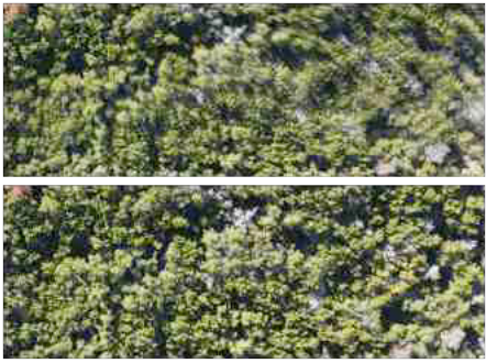
The system was tested on drone imagery of dense forest and tree canopy occasionally bisected by roads, using an uncalibrated lens. All computation proceeds at full image resolution, eliminating downsampling as a potential error source.

Application and Importance

Aerial image mosaicing serves numerous civilian and defense applications. In precision agriculture, mosaics of crop fields enable monitoring of vegetation health indices (NDVI) across spatial extents exceeding the field of view of any single exposure. In infrastructure inspection, mosaics of bridge decks, pipelines, and solar farms support automated defect detection. In cartography and land survey, orthomosaics produced from drone imagery have become a low-cost alternative to traditional aerial survey with accuracies approaching sub-decimeter GSD (ground sample distance).

In the defense and intelligence domains, aerial mosaics are foundational to geospatial intelligence (GEOINT) production. The National Geospatial-Intelligence Agency (NGA) integrates imagery intelligence (IMINT) mosaics with signals intelligence (SIGINT), electronic intelligence (ELINT), and communications intelligence (COMINT) for battle damage assessment, target tracking, pattern-of-life analysis, and broad-area situational awareness [3]. The proliferation of small UAS platforms has made wide-area persistent surveillance accessible at the tactical edge, where real-time onboard mosaicing can provide operators with a continuously updating composite image of the area of interest.

A key challenge in all these applications is that the mosaicing pipeline must tolerate imperfect sensor calibration, non-planar terrain, varying illumination, and atmospheric effects. The system described in this paper addresses these factors through a multi-stage registration and blending pipeline that adaptively refines alignment at progressively finer spatial scales.

Historical Context of the Methods

Area-Based Matching and NCC

Area-based image matching via cross-correlation was formalized by Pratt in 1974 for satellite image registration [4]. Lewis introduced fast normalized cross-correlation (NCC) in 1995, demonstrating that the normalization (which makes the metric invariant to linear brightness and contrast changes) can be computed efficiently using integral images [5]. NCC remains the standard metric for template matching in photogrammetric pipelines where feature-based methods (SIFT, ORB) are unavailable or inappropriate [6].

Lucas-Kanade Optical Flow

Lucas and Kanade introduced gradient-based iterative image registration in 1981, solving a local least-squares system (the 2 × 2 structure tensor) under the brightness constancy assumption [7]. Bouguet extended the method to a Gaussian image pyramid for handling large displacements [8]. The 6-DOF affine extension of Lucas-Kanade, which models rotation, scale, and shear in addition to translation, is the basis for the per-tile local deformation estimation used here.

Laplacian Pyramid Blending

Burt and Adelson [9] introduced multi-resolution spline blending in 1983, decomposing images into Laplacian pyramids (band-pass components at multiple octaves), blending each band with a transition zone matched to its spatial frequency, and collapsing the result. This eliminates the ghosting artifacts inherent in linear alpha blending while preserving fine detail. With well over 1,000 citations, the method remains the industry standard in panoramic stitching software.

Seam Finding

Efros and Freeman introduced minimum-error boundary cuts via dynamic programming for texture quilting in 2001 [10]. Kwatra et al. generalized the approach to graph-cut optimization for arbitrary-dimensional synthesis. In mosaicing, seam finding selects a connected path through the overlap region where the two images agree most closely, reducing the blending algorithm’s burden of masking residual misalignment [11].

Lens Distortion Modeling

Conrady first described the mathematics of tangential distortion from imperfect lens element alignment in 1919 [12]. Brown extended this to a unified polynomial model combining radial distortion (coefficients k1, k2) and tangential/decentering distortion (p1, p2). The Brown-Conrady model, formalized in Brown (1971) and later adopted by Tsai (1987) [27] and Zhang (2000) [28], is the basis of OpenCV’s camera calibration and virtually all modern photogrammetric toolkits [13,14].

Spatial Interpolation

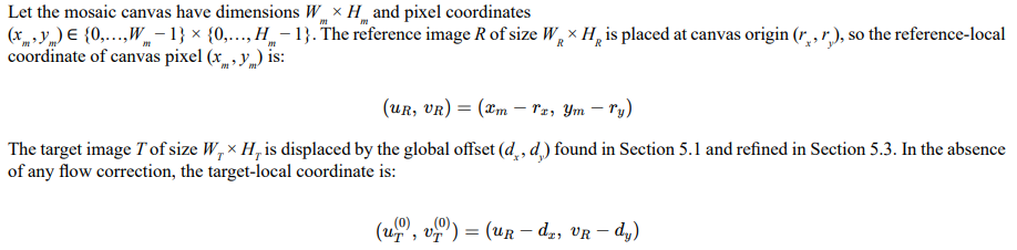
Shepard introduced inverse distance weighting (IDW) in 1968 for interpolating irregularly-spaced geographic data [15]. Catmull and Rom defined a family of C1-continuous cubic interpolating splines in 1974 that pass through all control points with automatically computed tangents [16]. Both methods are employed in the present pipeline: IDW for mesh-warp blending of tiled registration vectors, and Catmull-Rom splines for the final stage of flow field upsampling.

Implementation: Approaches Attempted and Abandoned

The development of the pipeline proceeded through several iterations in which specific algorithmic choices were evaluated and, when found deficient, replaced. This section documents the principal failure modes encountered and the reasoning behind each design change.

Bilinear Upsampling at Step=1 (Abandoned)

Initial per-pixel flow upsampling used bilinear interpolation directly from the 8-pixel flow grid to individual pixels. This produced paired-delta artifacts: at every other pixel along each axis, the interpolated flow exhibited a period-2 oscillation (stripe pattern) arising from the even/odd aliasing inherent in bilinear sampling with integer-spaced output and non-centered source coordinates. The symptom was fine vertical and horizontal striping visible in the mosaic, particularly in gradient-blend mode.

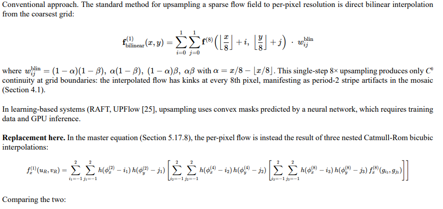
Resolution: Replaced with hierarchical upsampling (8 → 4 → 2 → 1) where each octave doubles the resolution using Catmull-Rom bicubic interpolation. At the final level ( step = 2 → 1), Catmull-Rom’s C¹ continuity eliminates the grid-boundary kinks that caused the period-2 artifacts.

Nearest-Neighbor Boundary Correction (Abandoned; Distance Field Retained)

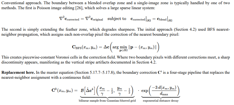
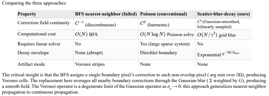
To correct color discontinuities at the boundary between the blended overlap zone and the single-image zone, the initial approach propagated the nearest boundary pixel’s color correction via breadth-first search (BFS). Each non-overlap pixel received the correction vector from whichever boundary pixel the BFS reached first. This created Voronoi-cell tessellations in the correction field: where two boundary pixels with different correction vectors met, a sharp discontinuity appeared as a visible vertical or horizontal stripe in the mosaic.

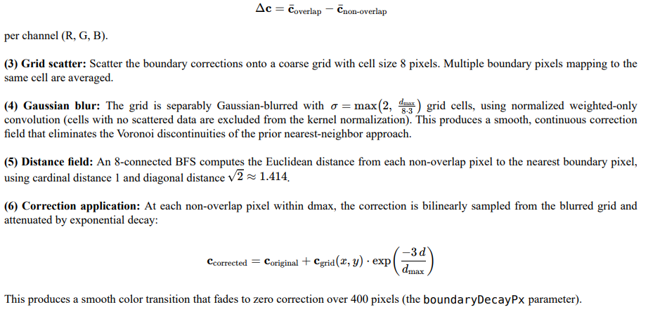
Resolution: Replaced with a C_o (Gaussian-smoothed, bilinearly sampled) correction grid. Boundary corrections are scattered onto a coarse grid (8 px cells), separably Gaussian-blurred, then bilinearly sampled at each non-overlap pixel with an exponential distance-decay envelope. The BFS is retained solely for computing the distance field used in the decay function.

Lucas-Kanade Micro-Refinement at Step=1 (Abandoned)

An attempt was made to run additional Lucas-Kanade refinement iterations at the per-pixel level (step = 1) after hierarchical upsampling. At this fine scale, the optimizer frequently fell into local minima in the high-frequency texture of forest canopy, introducing noise that was worse than the interpolated flow. The refinement was removed; the per-pixel flow is now obtained purely by interpolation from the 8-pixel-grid Lucas-Kanade solution.

Simple Flow Smoothing Without Root-Cause Fix (Abandoned)

Before the boundary correction mechanism was understood, extensive Gaussian smoothing was applied to the flow field itself in an attempt to suppress vertical stripe artifacts. While this reduced stripe visibility, it also degraded alignment quality in the overlap region. The smoothing was ineffective because the stripes originated in the boundary correction field, not in the flow field. Once the Gaussian-smoothed correction grid was implemented, no additional flow smoothing was required.

Final Process Flow and Detailed Mathematics

This section presents the complete pipeline as implemented in version 5 of the system. Each stage is described with its mathematical formulation.

Global Translation Estimation

Both images are downsampled to a maximum dimension of 400 pixels. A coarse exhaustive search evaluates the NCC at every 5-pixel offset within a radius of half the smaller image dimension, followed by a fine search at every integer pixel in a ±5-pixel neighborhood around the coarse optimum.

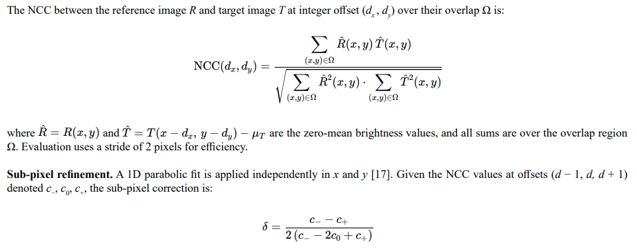
The correction is accepted only if |δ| < 1 and the denominator exceeds 10⁻³.

Two-Pass Tiled Registration

The overlap region is divided into a grid of tiles, first at coarse resolution (8 × 8 grid, 256-pixel half-width, pass 1) and then at fine resolution (12 × 12 grid, 96-pixel half-width, pass 2) targeting regions with high residual error. Each tile is matched by:

(a) Texture gate: The patch variance is computed from brightness samples at 4-pixel stride. Tiles with variance below 80 are rejected as low-texture.

(b) Coarse NCC search: Exhaustive search at 4-pixel stride within a ±30-pixel radius.

(c) Fine NCC search: Integer-pixel refinement in a ±4-pixel neighborhood around the coarse peak, evaluated at 2-pixel stride.

(d) Sub-pixel parabolic refinement: Identical to the global registration sub-pixel step.

(e) Affine Lucas-Kanade: Starting from the NCC translation, a 6-DOF affine model is iteratively refined using the Lucas-Kanade framework. The warp is parameterized as:

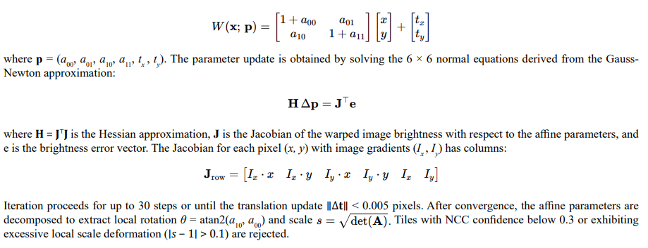
Global Offset Refinement from Tile Medians

After coarse tile registration, the median of the valid tiles’ residual displacements in ** and ** is computed. This median is added to the global offset, and the residuals are re-centered. This step separates the true lens distortion field (which is radially symmetric about the optical center) from a registration bias that would otherwise contaminate the distortion fit.

Robust Outlier Rejection via MAD

Outlier rejection uses the Median Absolute Deviation (MAD_n) [18, 19] applied independently to the x and y residual components. The normalized MAD estimator is:

MAD_n = 1.4826 ⋅ mediani |ri − medianj(rj)|

where the factor 1.4826 makes MAD_n a consistent estimator of the standard deviation under Gaussian noise. Tiles whose residual exceeds MADn from the median are rejected. A secondary spatial consistency check rejects tiles whose residual deviates from the mean of their neighbors (within 15% of the image diagonal) by more than max(3.0, 2.5 ⋅ MAD)..

Brown-Conrady Lens Distortion Fitting

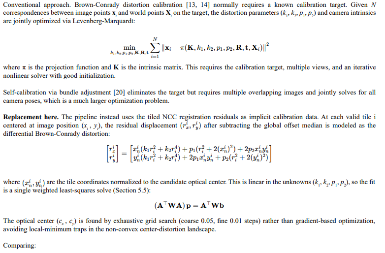
The lens distortion is modeled using the four-parameter Brown-Conrady model [13, 14] with radial coefficients k1, k2 and tangential coefficients p , p . For a point at normalized coordinates is the optical center and s = 1 max(W,H)/2, the distortion displacement is:

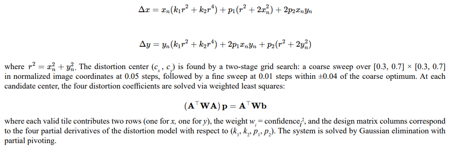
Dense Lucas-Kanade Optical Flow

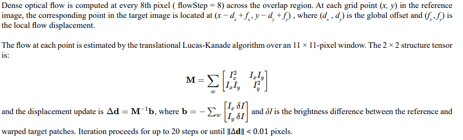
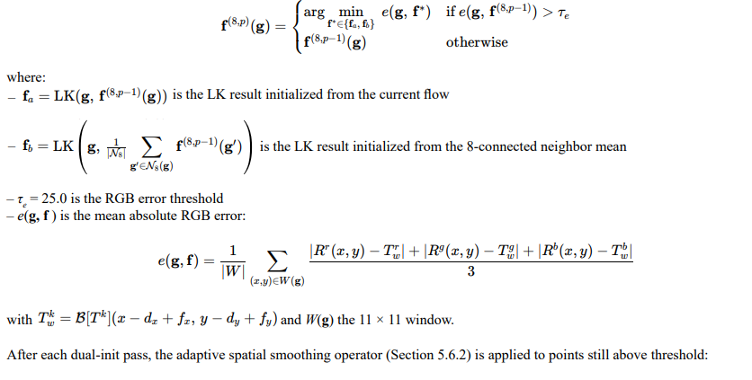
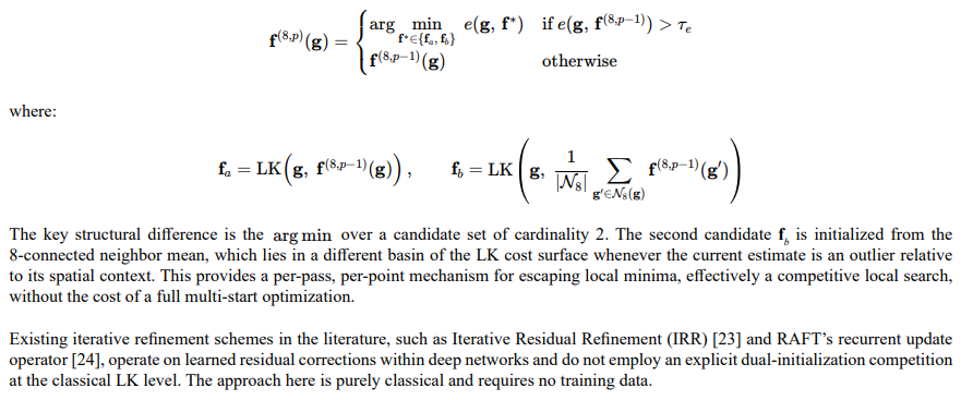
Iterative Dual-Initialization Refinement

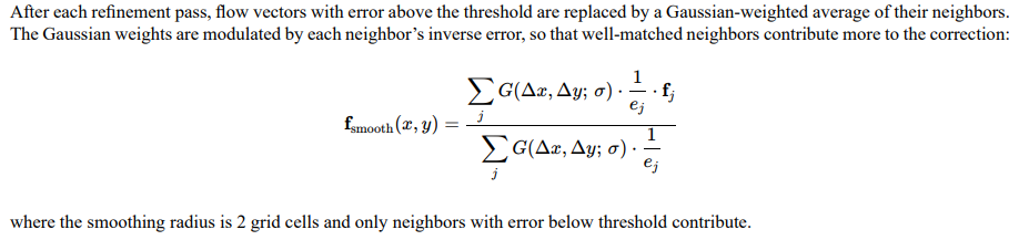
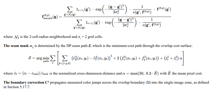
Adaptive Spatial Smoothing

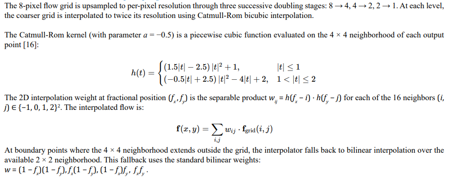
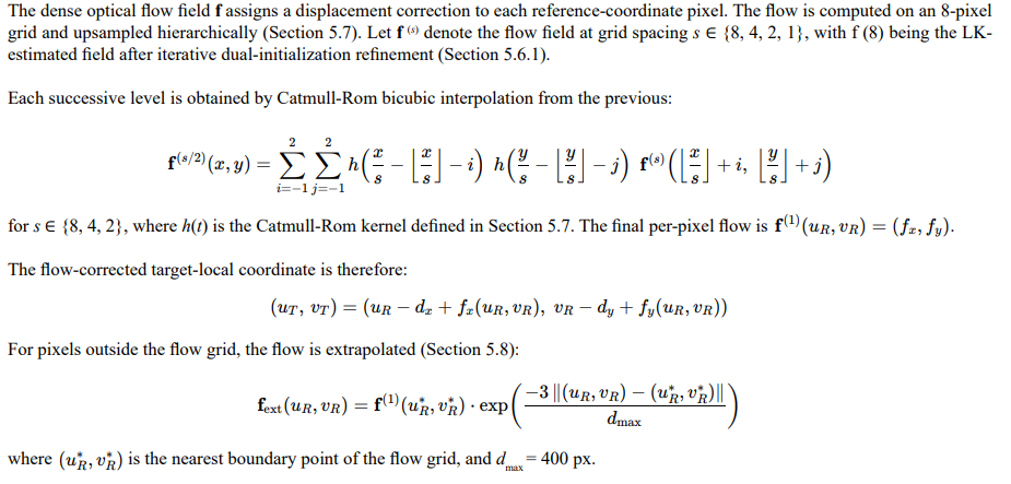
Hierarchical Per-Pixel Flow Upsampling

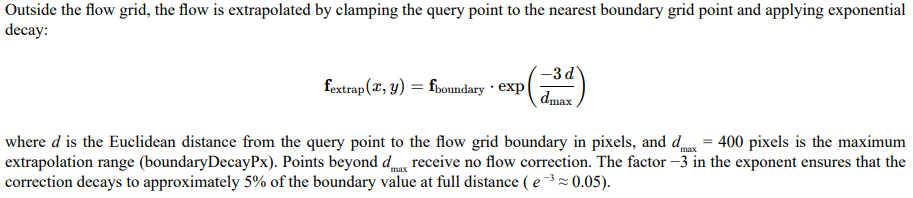
Flow Extrapolation Beyond the Overlap

Dynamic-Programming Seam Finding

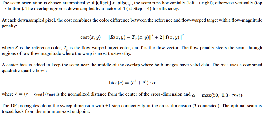
The downsampled path is upsampled to full resolution by linear interpolation between adjacent downsampled points, then smoothed by a box filter with a radius of 16 pixels to eliminate jagged staircase artifacts.

Mosaic Composition and Blending

The mosaic canvas is sized to span both images and is populated in two passes: the reference image is placed at its natural coordinates, and the target image is placed at the global offset with per-pixel flow correction applied. Flow correction uses the per-pixel arrays (pixFlowDX, pixFlowDY) when available, with fallback to bicubic interpolation from the 8-pixel grid via getFlowAtExtrap() for pixels outside the per-pixel coverage.

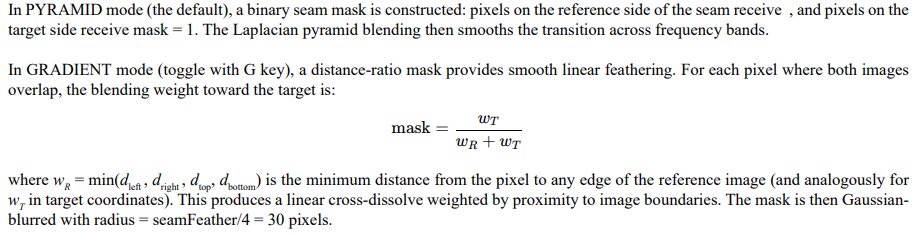
Blend Mask Construction

Source Fill for Black-Bleed Prevention

Before blending, pixels covered by only one source are filled with the other source’s color. This prevents black (zero) values from bleeding into the blend at the periphery of the overlap, which would create dark halos around the mosaic edges.

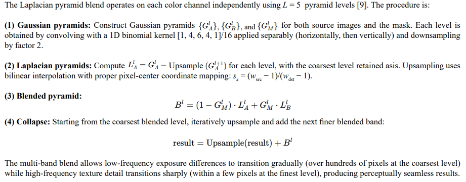
Laplacian Pyramid Multi-Band Blending

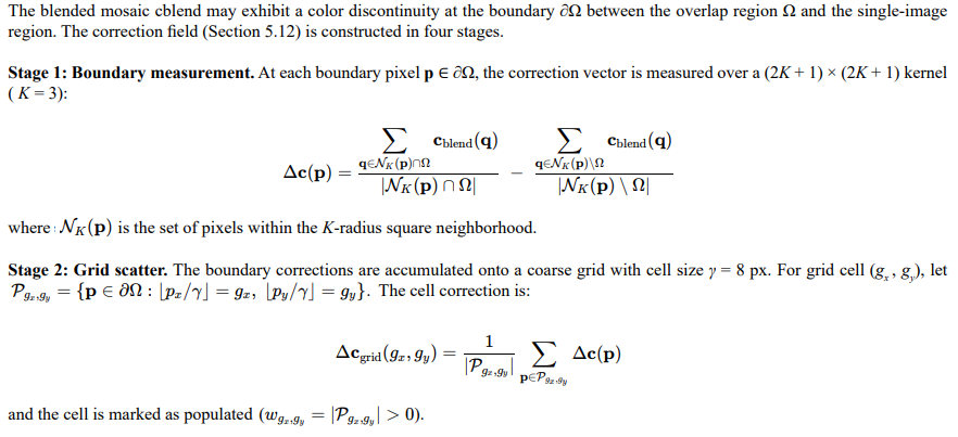
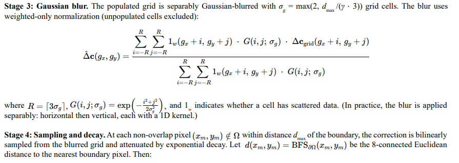
Gaussian-Smoothed Boundary Correction

The boundary between the blended overlap zone and the single-image zone can exhibit a color discontinuity because the blended overlap is a weighted mixture of two exposures while the adjacent single-image zone contains only one. The correction procedure is:

1.Boundary detection: Identify overlap pixels whose 4-connected neighborhood includes a non-overlap pixel.

2.Correction measurement: At each boundary pixel, measure the mean color on the overlap side and the non-overlap side within a 7× 7 kernel. The correction vector is the difference:

Mesh Warp Mosaic via IDW (Legacy Mode)

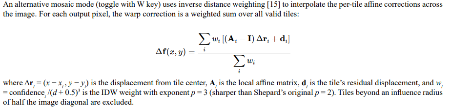
Image Distortion Correction

When calibration parameters are available (toggle with U key), both images are undistorted by inverse-mapping each output pixel through the Brown-Conrady model: for output pixel (x, y), compute the normalized coordinates, evaluate the distortion displacement (Δx, Δy) as in Section 5.5, and sample the input image at (x + Δx ⋅ s, y + Δy ⋅ s) using bilinear interpolation.

Bilinear Sampling

Linear System Solver

All linear systems ( 6 × 6 for affine LK, 4 × 4 for distortion fitting) are solved by Gaussian elimination with partial pivoting. The augmented matrix [A|b] is row-reduced; if the maximum pivot element falls below 10⁻¹⁴, the system is declared singular and the tile/fit is rejected. Back-substitution recovers the solution vector.

Unified Notation and the Master Equation

This section consolidates the per-stage formulations of Sections 5.1–5.16 into a single end-to-end expression that maps every output pixel in the final mosaic to the input pixels of the reference image R and the target image T . The master equation is developed in stages, first defining the coordinate transformations, then the per-pixel color contributions, and finally the complete output including boundary correction.

Coordinate Conventions

Per-Pixel Flow Correction

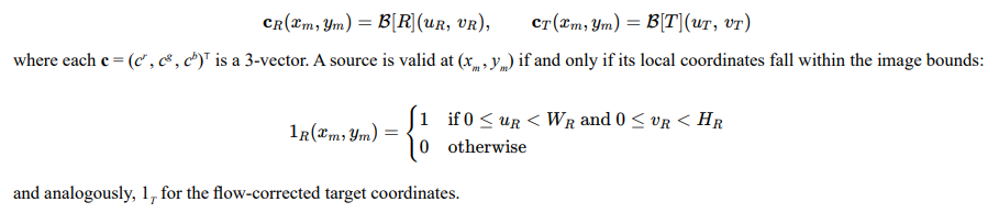
Source Color Sampling

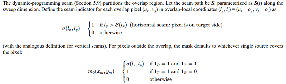
Seam Mask Construction

Laplacian Pyramid Blending Operator

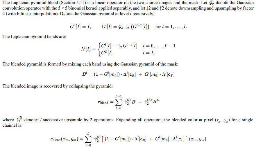
This is a linear combination of cR and cT with spatially varying, frequency-dependent weights determined by the mask pyramid {Gl[m0]}.

Source Fill (Black-Bleed Prevention)

Boundary Correction Field

The Master Equation

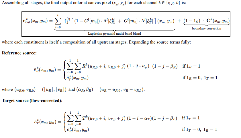
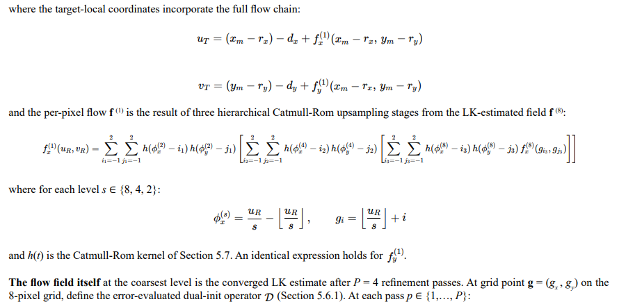
Summary: From Input Pair to Output Pixel

Symbol	Definition
πR	Reference projection: (xm, ym) → (xm − rx, ym − ry )
πT	Target projection: (uR, vR) → (uR − dx, vR − dy)
Φ	Per-pixel flow warp: (u, v) → (u + f (1)x, v + f (1) y), with f (1) from 3-stage Catmull-Rom upsample of f (8)
f (8)	Dense LK flow after P dual-init refinement passes with error-weighted smoothing
B~	Bilinear sampler with source-fill fallback (Section 5.17.6)
mS	Binary seam mask from DP with flow-magnitude + center-bias cost
L	L Laplacian pyramid blend: ∑ ↑(l) [(1 − Gl[m]) ⋅ Λl[⋅] + Gl[m] ⋅ Λl[⋅]] 2 l=0
E k ∂Ω	Boundary correction: scatter → Gaussian blur → bilinear sample → exponential decay
1Ω	Overlap indicator

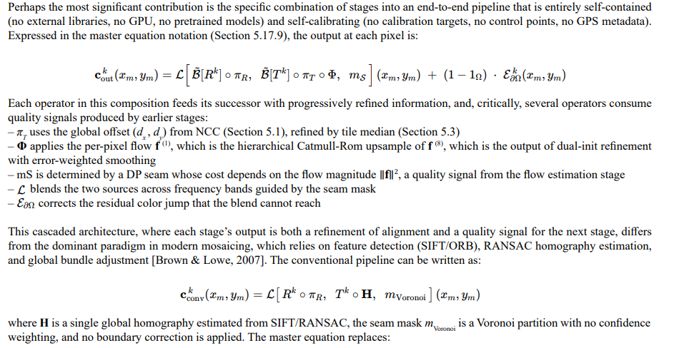
This master equation encodes the complete data path: every pixel of the output mosaic is a multi-scale, seam-guided, frequency-decomposed blend of bilinearly sampled source colors, where the target source coordinates are warped by a per-pixel flow field obtained through iterative dual-initialization Lucas-Kanade on an 8-pixel grid, hierarchically upsampled via three stages of Catmull-Rom bicubic interpolation, and where the boundary between the blended overlap zone and the single-image zone is healed by a Gaussian-smoothed, exponentially decaying correction field.

Statement of Novelty

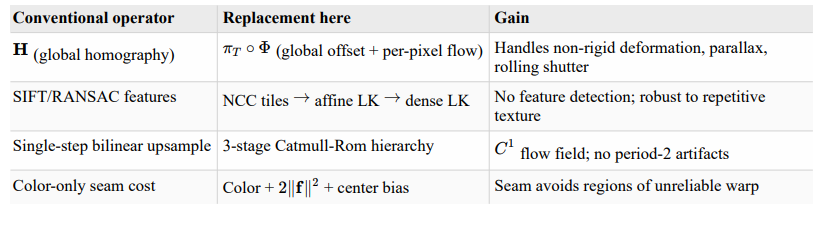
The pipeline described in this paper is, taken as a whole, a novel process for aerial image mosaicing. While individual components draw on established techniques, NCC [5], Lucas-Kanade optical flow, Brown-Conrady distortion modeling, Laplacian pyramid blending, and dynamic-programming seam finding [10], the system introduces six specific innovations and combines them into a self-contained, self-calibrating architecture that has no direct precedent in the literature [7,13,14,9,10]. This section identifies each novelty, states what conventional limitation it corrects, and summarizes the resulting advantage. Section 7 then provides the full comparative mathematics for each.

The Novel Process

Conventional aerial mosaicing pipelines follow a well-established sequence: detect sparse keypoints (SIFT, ORB), match them across images, estimate a global homography via RANSAC, and blend with a Voronoi or distance-weighted mask. This paradigm assumes that a single projective transformation adequately models the geometric relationship between images. In practice, uncalibrated consumer drone imagery violates this assumption due to lens distortion, terrain relief, wind-induced attitude changes, and rolling-shutter effects. The result is ghosting, misalignment in the overlap zone, visible seams, and abrupt color discontinuities at the overlap boundary.

The process introduced here replaces the global-homography paradigm with a dense, per-pixel registration cascade that is entirely feature-free, requires no calibration targets or GPS metadata, uses no external libraries or pretrained models, and runs on CPU in a single-file application. The pipeline progressively refines alignment through nine stages, from coarse global NCC through tiled affine tracking, self-calibrating distortion correction, dense optical flow with dual-initialization refinement, hierarchical Catmull-Rom upsampling, flow-aware seam finding, multi-band Laplacian blending, and scatter-blur-decay boundary correction, with each stage consuming quality signals produced by its predecessors.

Summary of Novel Contributions

The six specific innovations introduced by this pipeline, each of which corrects a concrete limitation of conventional methods, are:

Contribution 1: Dual-Initialization Iterative Flow Refinement

Problem corrected: Standard Lucas-Kanade flow refinement uses a single initialization per grid point. If the initial estimate sits in a poor local minimum of the brightness constancy cost surface, re-running LK from the same starting point returns the same minimum. In highly textured scenes such as forest canopy, a substantial fraction of grid points can become trapped.

Innovation: At each refinement pass, every high-error grid point is re-estimated from two independent initializations, the current flow and the 8-connected neighbor mean, and the result with lower photometric error is kept. This provides a per-point, per-pass mechanism for escaping local minima through competitive local search, without multi-start optimization or learned components.

Advantage: Reduces the number of outlier flow vectors in textured scenes without increasing computational cost by more than 2× per affected point. Unlike deep-network approaches (IRR, RAFT), this requires no training data and operates at the classical LK level.

Contribution 2: Error-Weighted Adaptive Spatial Smoothing

Problem corrected: Conventional flow smoothing (bilateral filtering, Horn-Schunck regularization) weights neighbors by image content, pixel intensity or gradient similarity. This preserves image edges but has no knowledge of whether a neighbor’s flow is actually correct. A neighbor with low photometric error and a neighbor with high photometric error contribute equally if their pixel intensities are similar.

Innovation: The smoothing kernel weights each neighbor by the inverse of its registration error ( 1/e) rather than by image similarity, and a hard gate excludes neighbors above the error threshold entirely. Smoothing is applied selectively, only to points still above the error threshold after dual-init refinement.

Advantage: The smoothing kernel is shaped by registration quality rather than image content. Well-aligned neighbors dominate; poorly aligned neighbors contribute negligibly regardless of texture similarity. This prevents bad flow from propagating through the field.

Contribution 3: Hierarchical Catmull-Rom Bicubic Flow Upsampling

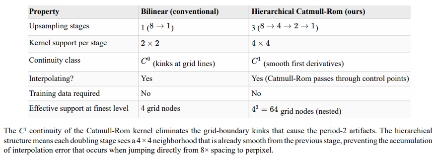
Problem corrected: The standard approach to upsampling a sparse flow field (computed on an 8-pixel grid) to per-pixel resolution is single-step bilinear interpolation. This produces only C0 continuity at grid boundaries, the interpolated flow has derivative discontinuities (kinks) at every 8th pixel, which manifest as visible period-2 stripe artifacts in the mosaic.

Innovation: The flow field is upsampled through three successive doubling stages ( 8 → 4 → 2 → 1), with each stage using Catmull-Rom bicubic interpolation over a 4 × 4 neighborhood. The Catmull-Rom kernel provides C1 continuity, smooth first derivatives, at every grid boundary.

Advantage: Eliminates the period-2 stripe artifacts caused by bilinear upsampling. The hierarchical structure ensures each doubling stage operates on an already-smooth field, preventing accumulation of interpolation error. No training data or GPU is required, unlike learned upsampling masks (RAFT [24], UPFlow [25]).

Contribution 4: Flow-Magnitude-Weighted Seam Cost

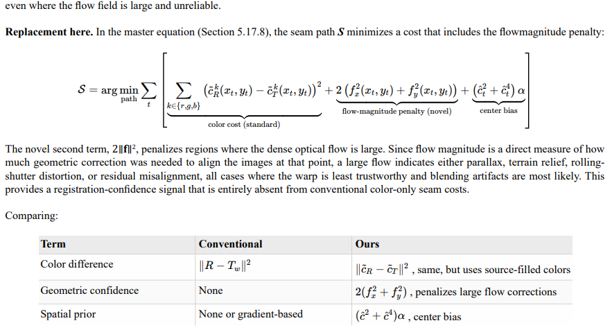
Problem corrected: Conventional dynamic-programming seam finding uses color difference as the sole cost term. This steers the seam toward regions where the two images happen to look similar, but provides no information about whether the geometric alignment is trustworthy at that location. In uniform-color regions (shadows, sky, dark canopy), the color cost can be low even where the flow field is large and unreliable.

Innovation: A flow-magnitude penalty term 2(f _x² + f _y²) is added to the DP cost function. Since flow magnitude directly measures how x y much geometric correction was needed at each pixel, large flow indicates parallax, terrain relief, rolling-shutter distortion, or residual misalignment, all cases where blending artifacts are most likely.

Advantage: The seam is steered through regions of minimal geometric correction, where the warp is most trustworthy, rather than merely through regions of similar color. This provides a registration-confidence signal that is entirely absent from conventional seam costs.

Contribution 5: Scatter-Blur-Decay Boundary Correction

Problem corrected: After blending the overlap zone, a color discontinuity typically remains at the boundary between the blended region (a weighted mixture of two exposures) and the adjacent single-image zone (one exposure only). Conventional solutions are either Poisson image editing (which requires solving a large sparse linear system) or extended feathering (which degrades sharpness). A simpler BFS nearest-neighbor approach was attempted but produced Voronoi-cell tessellations in the correction field, visible as sharp vertical stripe artifacts.

Innovation: Boundary color corrections are measured at each boundary pixel, scattered onto a coarse grid, Gaussian-blurred with weighted-only normalization, bilinearly sampled back to pixel resolution, and attenuated by exponential distance decay. This four-stage pipeline (scatter → blur → sample → decay) produces a smooth, continuous correction field without any linear solver.

Advantage: Eliminates the Voronoi discontinuities of nearest-neighbor propagation and the computational cost of Poisson solves. The Gaussian blur averages all nearby boundary corrections (rather than assigning the single nearest one), and the exponential decay provides a natural fade-to-zero envelope. The correction field is C0-continuous (smooth transitions without the Voronoi discontinuities of the prior approach, limited to C0 by the bilinear sampling step) and costs only O(N/gamma2) for a grid of cell size gamma.

Contribution 6: Self-Calibrating Distortion Fit from a Single Image Pair

Problem corrected: Brown-Conrady lens distortion calibration conventionally requires a known calibration target (checkerboard) photographed in multiple views, or bundle adjustment over many overlapping images. Neither is available when processing a single pair of drone photographs in the field without calibration infrastructure.

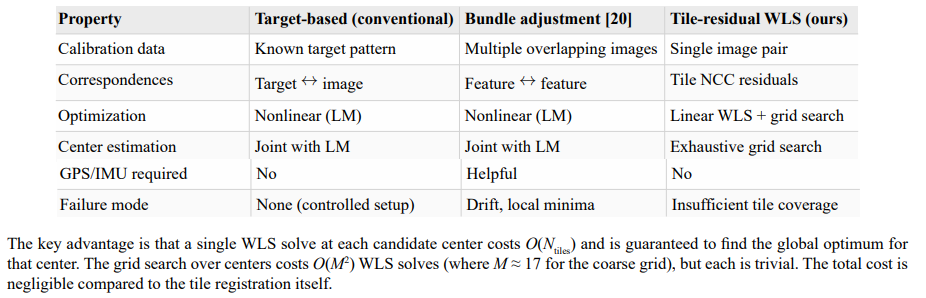
Innovation: The tiled NCC registration residuals, the displacement errors remaining after subtracting the global offset, are treated as implicit calibration data. Because the Brown-Conrady model is linear in the distortion coefficients (k1, k2, p1, p2) for a fixed optical center, the fit reduces to a single weighted least-squares solve. The optical center itself is found by exhaustive grid search over a coarse-then-fine grid, avoiding local-minimum traps in the non-convex center-distortion landscape.

Advantage: Calibrates the lens from a single image pair without calibration targets, GPS, or iterative nonlinear solvers. The grid search guarantees the global optimum for center location, and each WLS solve is O(Ntiles), negligible compared to the tile registration itself.

The Pipeline as a Novel Architecture

Beyond the six individual contributions, the pipeline architecture itself is novel in two respects:

Quality-signal cascading. Each stage produces not only a refined alignment but also a quality metric that the next stage consumes. The flow error drives the adaptive smoothing kernel; the flow magnitude drives the seam cost; the seam mask drives the Laplacian blend; the blend residual at the boundary drives the correction field. This cascaded quality-signal architecture differs fundamentally from the conventional detect-match-homography-blend pipeline, in which stages are largely independent.

Complete self-containment. The entire system, registration, calibration, flow estimation, seam finding, blending, and boundary correction, is implemented in a single application with no external libraries, no GPU dependencies, and no pretrained models. This makes the pipeline reproducible, auditable, and deployable in constrained environments (e.g., tactical edge computing) where library dependencies and GPU hardware may be unavailable.

Novel Contributions and Comparative Mathematics

While each individual technique in the pipeline draws on established methods, NCC [5], Lucas-Kanade [7], Brown-Conrady distortion [13, 14], Laplacian pyramid blending [9], dynamic-programming seam finding [10], several elements of this system are, to the author’s knowledge, novel in their specific formulation or in the way they are combined. This section identifies each novel contribution, states the conventional formulation it replaces, derives the replacement in the unified notation of Section 5.17, and explains why the substitution improves the result [5,7,13,14,9].

Dual-Initialization Iterative Flow Refinement

Conventional approach. Standard Lucas-Kanade optical flow estimation uses a single initialization per grid point, either zero or coarse-to-fine propagation from a pyramid level above [8]. The conventional iterative refinement at pass p is:

This re-runs LK from the previous estimate. If the previous estimate sits in a poor local minimum of the brightness constancy objective, the refinement returns the same minimum, there is no mechanism for escape.

Replacement here. In the master equation (Section 5.17.8), the flow at each grid point is instead determined by the dual-initialization operator:

Error-Weighted Adaptive Spatial Smoothing

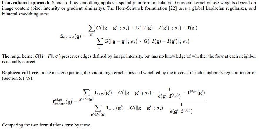
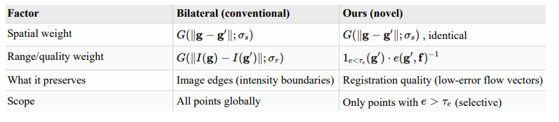
The critical substitution is replacing the intensity-based range kernel with the inverse warp error 1/e. This means the smoothing kernel is shaped by how well each neighbor’s flow actually aligns the images, not by whether the underlying image content is similar. A neighbor with perfect alignment ( e → 0) dominates; a neighbor that is itself poorly matched contributes negligibly, regardless of image similarity. The hard gate 1_e<τe further excludes neighbors above the error threshold, preventing bad flow from propagating.

Hierarchical Catmull-Rom Flow Upsampling

Flow-Magnitude-Weighted Seam Cost

Gaussian-Smoothed Boundary Correction Field

Self-Calibrating Distortion Fit via Grid-Search-Initialized WLS

The Pipeline as a Whole

Future Work

Multi-Image Mosaicing ( N > 2)

The current system operates on exactly two images. Extension to N > 2 images requires: (a) pairwise registration of all overlapping pairs, (b) global bundle adjustment to jointly optimize all camera parameters and minimize cumulative drift, (c) a global seam-finding strategy (e.g., Voronoi-based label assignment with graph-cut optimization [11]) to partition the output canvas among N sources, and (d) multi-image Laplacian pyramid blending with per-pixel source selection [20]. The Brown-Conrady distortion calibration generalizes naturally to multi-image scenarios: the same distortion parameters apply to all images from the same camera, providing a strong cross-image constraint. Bundle adjustment could employ Levenberg-Marquardt optimization over the joint set of global offsets, per-pair flow fields, and the shared distortion model.

Wide Spectral Range Matching

Matching images from different spectral bands (e.g., visible RGB against near-infrared, thermal infrared, or synthetic aperture radar) requires replacing the NCC metric, which assumes correlated brightness, with a modality-invariant similarity measure. Mutual information (MI), which measures the statistical dependence between intensity distributions, has been shown effective for multi-modal registration [21]. Alternatively, structural descriptors such as the Modality-Independent Neighborhood Descriptor (MIND) or learned feature embeddings from cross-spectral matching networks could serve as the matching cost in both the tile-registration and dense-flow stages. The Laplacian pyramid blending would require adaptation to handle different dynamic ranges and radiometric responses across bands.

Integration into SIGINT Workflows

Aerial image mosaics provide the spatial reference layer onto which signals intelligence products are geo-registered. Integration into a SIGINT workflow would involve: (a) geotagging each mosaic pixel using the drone’s GPS/IMU telemetry and the computed registration transforms, producing an orthorectified georeferenced mosaic; (b) fusing the mosaic with RF sensor geolocation data (e.g., TDoA emitter positions from onboard COMINT/ELINT payloads [3]) by projecting emitter coordinates onto the mosaic canvas; (c) enabling temporal mosaicing for change detection and pattern-of-life analysis; and (d) implementing real-time incremental mosaicing for onboard processing on edge computing platforms, potentially leveraging GPU-accelerated flow computation. The pipeline’s self-calibrating nature (no external calibration targets required) makes it suitable for field deployment where calibration infrastructure is unavailable.

Further integration could include automated object detection and geotagging (applying convolutional neural networks to the mosaic for vehicle, structure, or anomaly detection), mosaic-based GMTI (ground moving target indication) by differencing temporally adjacent mosaics, and multi-INT fusion where IMINT mosaics, SIGINT geolocation ellipses, and HUMINT report locations are composited into a unified common operating picture.

Final Notes

The most instructive lesson from the development process was that visible artifacts (vertical stripe patterns) often have root causes far removed from where they manifest. The stripes appeared in the final mosaic and were initially attributed to the flow field, the pyramid blending, or the seam finding. Extensive diagnostic instrumentation, including per-stage pipeline image exports, flow field visualizations, and selective disabling of pipeline components, eventually traced the cause to the boundary correction field and its Voronoi-cell discontinuity structure. The fix was straightforward (Gaussian blur of a scattered correction grid), but identifying the root cause required systematic elimination of hypotheses across a 10-stage pipeline [22-26].

The combination of multi-scale NCC registration, iterative affine Lucas-Kanade refinement, dense optical flow with hierarchical upsampling, seam-guided Laplacian pyramid blending, and Gaussian-smoothed boundary correction produces visually seamless mosaics from uncalibrated consumer drone imagery without requiring external calibration targets, control points, or GPS metadata.

References

- Polidori, L. (2020). On Laussedat’s contribution to the emergence of photogrammetry. The International Archives of thePhotogrammetry, Remote Sensing and Spatial Information Sciences, 43, 893-899.
- Szeliski, R. (2007). Image alignment and stitching: A tutorial. Foundations and trends in computer graphics and vision, 2(1), 1-104.
- Harbaugh, M. (2018). “Unmanned Aerial Systems (UAS) for Intelligence, Surveillance and Reconnaissance (ISR).” DSIAC State-of-the-Art Report DSIAC-2018-0849.
- Pratt, W. K. (2007). Correlation techniques of image registration. IEEE transactions on Aerospace and Electronic Systems, (3), 353-358.
- Lewis, J. P. (1995, May). Fast normalized cross-correlation. In Vision interface (Vol. 10, No. 1, pp. 120-123).
- Lowe, D. G. (2004). Distinctive image features from scale-invariant keypoints. International journal of computer vision, 60(2), 91-110.
- Lucas, B. D., & Kanade, T. (1981, August). An iterative image registration technique with an application to stereo vision. In IJCAI’81: 7th international joint conference on Artificial intelligence (Vol. 2, pp. 674-679).
- Bouguet, J. Y. (2001). Pyramidal implementation of the affine lucas kanade feature tracker description of the algorithm. Intel corporation, 5(1-10), 4.
- Burt, P. J., & Adelson, E. H. (1983). A multiresolution spline with application to image mosaics. ACM Transactions on Graphics (ToG), 2(4), 217-236.
- Efros, A. A., & Freeman, W. T. (2023). Image quilting for texture synthesis and transfer. In Seminal Graphics Papers: Pushing the Boundaries, Volume 2 (pp. 571-576).
- Kwatra, V., Schödl, A., Essa, I., Turk, G., & Bobick, A. (2003). Graphcut textures: Image and video synthesis using graph cuts. Acm transactions on graphics (tog), 22(3), 277-286.
- Conrady, A. E. (1919). Decentred lens-systems. Monthly notices of the royal astronomical society, 79(5), 384-390.
- Brown, D. (1996). Decentering distortion of lenses. Photogrammetric engineering, 32(3), 444-462.
- Brown, D. C. (1971). Close-range camera calibration. Photogrammetric engineering, 37(8), 855-866.
- Shepard, D. (1968, January). A two-dimensional interpolation function for irregularly-spaced data. In Proceedings of the 1968 23rd ACM national conference (pp. 517-524).
- Catmull, E., & Rom, R. (1974). A class of local interpolating splines. In Computer aided geometric design (pp. 317-326). academic Press.
- Fisher, R. B., & Naidu, D. K. (1996). A comparison of algorithms for subpixel peak detection. In Image Technology: Advances in Image Processing, Multimedia and Machine Vision (pp. 385-404). Berlin, Heidelberg: Springer Berlin Heidelberg.
- Hampel, F. R. (1974). The influence curve and its role in robust estimation. Journal of the american statistical association, 69(346), 383-393.
- Rousseeuw, P. J., & Croux, C. (1993). Alternatives to the median absolute deviation. Journal of the American Statistical association, 88(424), 1273-1283.
- Brown, M., & Lowe, D. G. (2007). Automatic panoramic image stitching using invariant features. International journal of computer vision, 74(1), 59-73.
- Viola, P., & Wells III, W. M. (1997). Alignment by maximization of mutual information. International journal of computer vision, 24(2), 137-154.
- Horn, B.K.P. and Schunck, B.G. (1981). “Determining Optical Flow.” Artificial Intelligence, vol. 17, no. 1-3, pp. 185-203.
- Hur, J. and Roth, S. (2019). “Iterative Residual Refinement for Joint Optical Flow and Occlusion Estimation.” Proc. CVPR, pp. 5754-5763.
- Teed, Z. and Deng, J. (2020). “RAFT: Recurrent All-Pairs Field Transforms for Optical Flow.” Proc. ECCV, pp. 402-419.
- Luo, K., Wang, C., Liu, S., Fan, H., Wang, J., and Sun, J. (2021). “UPFlow: Upsampling Pyramid for Unsupervised Optical Flow Learning.” Proc. CVPR, pp. 1045-1054.
- Perez, P., Gangnet, M., and Blake, A. (2003). “Poisson Image Editing.” ACM Trans. Graphics (SIGGRAPH), vol. 22, no. 3, pp. 313-318.
- Tsai, R.Y. (1987). “A Versatile Camera Calibration Technique for High-Accuracy 3D Machine Vision Metrology Using Off-the-Shelf TV Cameras and Lenses.” IEEE J. Robotics and Automation, vol. 3, no. 4, pp. 323-344.
- Zhang, Z. (2000). “A Flexible New Technique for Camera Calibration.” IEEE Trans. Pattern Analysis and Machine Intelligence,vol. 22, no. 11, pp. 1330-1334.