Deep Learning-Based Trading Strategy for Index ETFs Using LSTM and GARCH Under Market Uncertainty

Introduction

Most of the literature has focused on Index ETFs being part of the investment portfolios due to their low cost and strong liquidity. This is an advantage when you want diversification in your portfolio. The early research has focused on GARCH-type models, as seen in works such as GARCH-type models to capture volatility patterns and inform trading decisions [1-5]. Researchers and investors focus more on developing new strategies that will enable effective trading of index EFTs. The approach being used has assumptions such as smooth volatility dynamics, and this might not work when dealing with sudden changes in market disruption, such as policy changes or geopolitical tensions by Dabrowski [6]. The traditional model, such as momentum strategies, performed poorly during the period of the COVID-19 pandemic due to rapid changes in the market, resulting in significant losses in the short positions, as the work done by Rericha shows that declining stocks rebounded sharply [7].

The work done by Sepp and Jurgen introduces the models that address the shortcomings of the traditional models when we have a market that is uncertain. In their work introduce deep learning architectures such as LSTM networks [8]. Another approach was done by Vaswani and Shazee to address the above issue using the Transformers model. LSTM networks assist in capturing the long¬term dependencies in time series through the gating mechanisms [9]. Transformer models are different from LSTM and were initially introduced for natural language processing tasks. that uses self-attention to model both short and long-range relationships in an organized manner through parallel processing. These capabilities let LSTM and Transformer models better assist in capturing the nonlinearities and unexpected changes that form the market uncertainty. The literature has focused mostly on the approaches that use LSTM and Transformers for financial time series forecasting and risk modeling. In particular, LSTM has shown an improved predictive accuracy when compared with existing models such as logistic regression and ARIMA [10, 11]. Another method that has pick the interest of researchers and traders is Transformer-based approaches, which have shown strong performance in financial forecasting by effectively modeling long-range dependencies and multivariate series [12,13]. Beyond individual architectures,

hybrid methods that combine both deep learning models with econometric volatility measures, such as GARCH, have also been proposed to improve the accuracy and enable the model to be able to adapt under stressful markets, see the work done by [14-16]. Recent research done in this direction showed that integrated market uncertainty indicators, including the Economic Policy Uncertainty (EPU) index and the VIX, into forecasting models have better performance under regime shifts and external shocks, see the results obtained in [17-20].

We propose a hybrid trading strategy that combines deep learning classifiers (e.g., LSTM, feedforward networks) with volatility features derived from multiple GARCH-family models (GARCH, EGARCH, GJR-GARCH, APARCH, IGARCH). Rather than using these econometric models for direct prediction, we use their estimated volatilities as input features to improve the deep learning model’s ability to anticipate price movements. This setup allows the model to learn from both historical price patterns and risk dynamics captured by volatility modeling.

Literature Review

Deep Learning for Time Series Forecasting

Deep learning models in the previous years have had success in financial time series forecasting. This section will review the application of using both the LSTM networks and Transformer models to model market dynamics, as well as current efforts to combine deep learning with the traditional econometric models through hybrid architectures.

LSTM Networks

Most of the literature has focused on using the LSTM model for market forecasting. One of the examples we can use is the Chinese stock market, which showed that the LSTM-based prediction can achieve higher returns when compared to the random forecasting strategies. Fischer and Krauss have built on this idea by showing that LSTMs can outperform conventional models such as logistic regression and random forest using the S&P 500 stocks to predict the returns [22]. The research in this direction has explored the architectural improvements to improve the predictive performance. For instance, Zou et al. in their results have suggested that stacked-LSTM models show stronger forecasting capabilities when compared to other LSTM variants [23].

Besides focusing on the improvement of the returns of the assets, there has been conducted to check the underlying reasons why the LSTM has the superior performance. Nelson et al. showed that the LSTM networks are particularly useful when applied to modeling nonlinear patterns of financial time series, outperforming traditional approaches such as Autoregressive Integrated Moving Average (ARIMA) and multilayer perceptrons (MLPs) [24]. Gowani and Kanjiani have extended the study to explore the sector-level analysis by applying LSTMs to nine sector ETFs and, as a result, showed that they achieve an average R2 of 0.865 and a peak around 0.942 for VNQ. This shows that LSTMs can effectively capture sector-specific trends that are critical to ETF trading [25].

We have that the practical implementation has focused on the importance of the trading strategy designed, which is beyond the predictive accuracy of the asset return. Silva et al. have used the five-minute trading strategy and showed that an LSTM-based trading system has achieved a return of around 220% despite the low forecasting precision, and this highlights the important role rule adherence and risk control play in trading systems [26].

Transformer Models

Transformer models were originally introduced to be used for natural language processing work. Their attention-based architecture has also made them suitable to model the long-range dependencies and multivariate time series. Muhammad et al. applied a Transformer model to the Bangladesh stock market and reported an improved return accuracy compared to the ARIMA as the benchmark. This shows that the applications of the transformers, when applied to the financial markets, show promising results. Wang et al used the Transformer model to forecast major stocks market indices and it showed that it also captures underlying market dynamics as LSTM above, outperforming deep learning approaches such as the convolutional neural network (CNNs) and LSTMs. Ding et al. have introduced the modifications that include the multi-scale Gaussian prior, orthogonal regularization, and a trading gap splitter, and using the NASDAQ have achieved a good performance when compared to just ARIMA. The Transformation has assisted with addressing the complexities of the financial time series. Tuncer et al. have explored the attention mechanisms that are beyond the sequential modeling, and their approach is transforming the financial data into images, which allows them to apply the vision transformers. Their proposed model has delivered strong, sharp ratios and shows returns for different ETFs [27-30].

Hybrid Architectures

Hybrid modeling approaches aim to use the strengths of different models. The model can be a combination of traditional or deep learning models to obtain even stronger prediction power. Scott and Nicholas, have shown that when you combine the GARCH models, which are effective when capturing the volatility of assets, and the combination with the LSTM leads to an improved volatility prediction accuracy [11]. Bao and Yue proposed the hybrid modeling, which is beyond the study of volatility modeling, and in their paper have introduced the combination of wavelet transforms, stacked autoencoders, and LSTM networks, which is used to do the stock price forecasting. They obtain higher accuracy across the six major stock indices when compared to traditional methods, such as LTSM individually [2]. Takeuchi and Lee in their paper have developed a hybrid method by using stacked restricted Boltzmann machines (RBMs) method for feature extraction along with the neural network classifier, resulting in an annual return which is around 45.93% for the period 1990–2009 which shows the performance of the model and it outperform basic momentum strategies [26]. The recent work done by Kabir et al. has introduced the LSTM-mTrans-MLP, which is a hybrid architecture that combines the LSTM networks, a modified version of the Transformer design, and the multilayer perceptions (MLPs), which shows the forecasting accuracy across different financial assets, including cryptocurrency such as Bitcoin [16].

Risk Forecasting and Market Uncertainty Modeling

Risk forecasting and market uncertainty modeling play an important role in making decisions in financial and portfolio management. This section will discuss the traditional volatility modeling approaches, such as the methods of GARCH and the extension, which is EGARCH. Recently, studies have been conducted in hybrid models combining both deep learning and statistical indicators from econometrics.

Risk Forecasting

Volatility forecasting has long been an important component for risk management in financial markets, as it is used as a volatility prediction and give accurate directly influences asset pricing and the development of trading strategies. Early econometric models, particularly those in the GARCH family, have been widely adopted to model time-varying volatility [9]. Engle in their paper have introduced the Autoregressive Conditional Heteroskedasticity (ARCH) model, which was later Bollerslev generalized the method who is now called the Generalized ARCH (GARCH) model. These models are effective in capturing volatility clustering and have become foundational tools for forecasting Value-at-Risk (VaR). Engle and Manganelli have introduced the quantile-based methods, which are an extension to improve the limitations of the traditional models. Furthermore, they introduce the conditional autoregressive value at risk(CAViaR) model, which assists with estimating the VaR through the quantile regression rather than using the assumption of specific volatility dynamics [10]. This approach gives flexibility in risk forecasting.

Roszyk and Slepaczuk have shown that the LSTM-GARCH models outperform the GARCH models, particularly in the case where the markets are volatile, by capturing both long-term dependencies and short-term volatility shocks. Pan et al. have combined the GARCH- based volatility features into LSTM networks, resulting in high accuracy prediction under the condition of the stressed market [14]. There is ongoing research on financial risk management that emphasizes the importance of a model to be able to adjust in real-time to uncertainty [18]. Silva et al. have shown that when we have relatively low predictive accuracy, the application of the volatility-based risk controls can yield substantial trading returns. Combining these studies, it has demonstrated that adding the econometric volatility forecasting with deep learning models provides a good direction for improving risk-sensitive trading strategies, particularly in the case of high market uncertainty [25].

Market Uncertainty Modeling

Market uncertainty comes from factors such as policy changes, geopolitical risks, and investor sentiment, which have an impact on the financial markets. Baker, Bloom, and Davis introduced the Economic Policy Uncertainty (EPU) index, which is used to measure the policy-related issues, such as the news coverage [17]. This approach has quantified and helped in analyzing uncertainty. In their result, they have found that the elevated EPU levels are correlated with reduced investment and hiring. This result highlights the impact of the economy on policy uncertainty. For the real-time market, we use the Volatility(VIX), which plays a role in assisting in estimating the expected volatility. The VIX captures a lot of market participants, the expectation of near-term volatility, and assists in providing insights into the market sentiment during the period of market stress.

Hamilton proposed the Markov switching model to assist in modeling the dynamic nature of the financial markets [18]. This approach allows for regime changes in the time switching model. The results are that it can capture effectively the shifts between different market conditions, such as bull and bear markets. This also includes the probabilities of transitioning between regimes. Wood et al. have developed a trading strategy that combines deep learning with the changepoint detection. This approach allows him to enabling the model to predict with high accuracy in sudden market shifts, and this leads to improved performance during volatile periods [30].

Experiments

This paper examines the predictive performance and trading performance of a hybrid LSTM-GARCH model on SPY ETF (S&P 500) data. We consider the following three approaches for evaluation:

• Buy-and-hold strategy

• Stand-alone LSTM-based prediction

• LSTM with GARCH-based volatility features

Predictive performance is evaluated in terms of mean absolute error (MAE) and root mean squared error (RMSE) of next-day returns, and trading performance is evaluated in terms of annualized return, Sharpe ratio, and maximum drawdown, with the aid of backtesting results.

We apply a volatility regime analysis using Hidden Markov Models (HMMs) to evaluate model performance across low- , medium-, and high-volatility periods. To account for changing market conditions over time. Expected Outcomes: The hybrid approach, combining time-series forecasting with LSTMs and volatility-based information with GARCH models, would offer superior predictive performance and risk-adjusted returns compared to the LSTM-only and buy-and-hold benchmarks.

Methodology

We propose a hybrid trading strategy that combines deep learning and econometric volatility modeling to forecast price movements for the SPY ETF under market uncertainty. We implement a Long Short-Term Memory (LSTM) network that incorporates volatility estimates from GARCH-family models (including EGARCH, APARCH, GJR-GARCH, and IGARCH) as additional input features. Technical indicators such as RSI and MACD, as well as regime-switching information from a 3-state Hidden Markov Model (HMM), are also integrated into the model.

We compare the performance of a pure LSTM model against a hybrid LSTMGARCH model using next-day return classification and backtesting a simple discrete trading strategy based on the predicted direction of returns. Evaluation metrics include accuracy, Sharpe ratio, and drawdown. Although Transformer models and multi-ETF evaluation are noted for future exploration, the current implementation focuses on forecasting the SPY ETF.

Model Architecture Overview

The proposed hybrid model integrates deep learning and econometric volatility modeling to enhance directional forecasting and risk-sensitive decision making in SPDR S&P 500 ETF Trust (SPY) trading. The architecture consists of three main components: a GARCH-family volatility estimator, a deep learning classifier (LSTM or DNN), and a rule-based trading strategy derived from classification outputs. The method uses five models from the GARCH family—GARCH(1,1), EGARCH(1,1), GJR-GARCH(1,1), APARCH(1,1), and IGARCH(1,1) to estimate conditional volatility, based on which it calculates volatility-adjusted returns. Gaussian Hidden Markov Models (HMMs) identify market regimes on raw as well as volatility-adjusted returns. Technical indicators such as the Relative Strength Index (RSI) and Moving Average Convergence Divergence (MACD) are computed and discretized into trading signals. The deep learning models (LSTM and feedforward DNN)are trained on a fusion of these features, such as returns, technical indicators, GARCH volatilities, and HMM regimes. This transparent and modular arrangement substitutes the initial Transformer and model fusion recommendation with a more interpretable and focused pipeline that incorporates the econometric output along with the machine learning classification to aid real-time trading decisions.

Data Sources

This study utilizes daily open, high, low, close, volume data for the SPDR S&P 500 ETF Trust (SPY), sourced from Yahoo Finance using they finance Python library. This dataset provides a reliable foundation for modeling market dynamics and volatility patterns over time.

Time period

The dataset spans from January 2010 to December 2024, capturing several key market phases, including the post-2008 recovery period, the 2020 COVID-19 market crash, and the inflation-driven regime shifts of 2022–2023. This time frame ensures a comprehensive view of various market regimes and their impact on financial models.

Preprocessing Steps

Data preprocessing included handling missing values through forward-fill and linear interpolation methods to maintain temporal consistency. Log returns were computed from the adjusted close prices to eliminate long-term trends and stabilize variance. The formula used is:

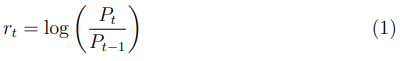
where Pt denotes the closing price on day t. To further enhance model training and ensure robustness, features were standardized using the StandardScaler from the scikit-learn library, which transforms data to have zero mean and unit variance based solely on the training set. This prevents data leakage and look-ahead bias often caused by rolling statistical measures.

Data Frequency

A daily frequency was selected to strike a balance between capturing the responsiveness of market movements and minimizing noise, especially for volatility modeling purposes.

We used the arch library in Python to build and compare five different GARCH models to track how market volatility changes over time. All models were fitted to the daily return series of the SPY ETF, and their conditional volatility outputs were retained as features to be utilized for downstream modeling.

The models implemented in this study include several variations of GARCH models designed to capture different aspects of financial time series volatility.

GARCH(1,1) is a symmetric model that captures volatility clustering, where large changes in returns tend to be followed by large changes (of either sign), and small changes tend to be followed by small changes.

EGARCH(1,1) extends the basic GARCH model by accounting for asymmetric effects, commonly known as the leverage effect, where negative shocks may have a larger impact on volatility than positive ones.

GJR-GARCH(1,1) introduces threshold terms that allow the model to differentiate between the effects of positive and negative shocks on volatility, further enhancing asymmetry modeling.

APARCH(1,1) generalizes the GARCH model by incorporating both asymmetry and power transformations of the standard deviation, offering greater flexibility in fitting volatility patterns.

IGARCH(1,1) assumes that shocks have a permanent effect on future volatility, implying complete persistence and no mean reversion in the variance process.

Maximum likelihood was used to estimate all models. The conditional volatilities of the models were saved in different columns of the data. An example of the standard GARCH(1,1) model specification is shown below:

The EGARCH volatility equation takes a logarithmic form to allow for negative coefficients and asymmetric effects:

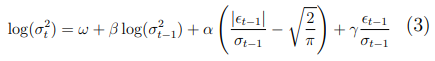
The conditional volatility output from each model was stored as a separate column in the dataset. These volatility estimates were later used in both the classification model and regime detection processes (e.g., HMM applied to GARCH-adjusted returns).

We also calculated volatility-adjusted returns by dividing the raw return series by the corresponding conditional volatility. This helped normalize the return distribution over time and supported better learning performance in downstream neural network models.

Volatility-adjusted returns as:

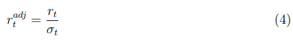
σt : the conditional volatility obtained from the GARCH(1,1) model. They were used as explanatory variables by the deep learning classifiers (DNN and LSTM). They were utilized as inputs to Hidden Markov Models (HMM) for the detection of market regimes.

Deep Learning Module (LSTM)

The deep learning module is tasked with capturing the nonlinear dependencies and temporal dynamics of the feature set. There were two categories of neural networks in our work

• LSTM (Long Short-Term Memory)

• Feedforward Deep Neural Network (DNN)

These models took multivariate inputs such as raw and adjusted returns, GARCH volatilities, HMM-based regime labels, technical signals (e.g., RSI, MACD). The response variable was a 3-class label (down, neutral, up) derived from next-day returns.

The model takes multivariate features as input, including volatility, returns, HMM regimes, MACD, and RSI indicators. Its output is a class label predicting the directional return. For training, the model uses either sparse categorical cross-entropy or categorical cross¬entropy as the loss function. The purpose is to Predict short-term direction of returns to assist trading decisions (Buy, Hold) [31].

Regime Detection with Hidden Markov Models

We utilized Gaussian Hidden Markov Models (HMMs) available in the hmm learn package to identify hidden market regimes.The models were set with three hidden states that correspond to qualitatively different regimes of market volatility: low, moderate, and high volatility. Two HMM architectures were trained:

• One based on raw return series

• One based on volatility-adjusted returns (obtained from the GARCH(1,1) model)

Predicted regime labels (integer values: 0, 1, 2) were saved as features and subsequently utilized by the deep learning classifiers for learning regime sensitive dynamics.

Feature Engineering

To enhance the model’s predictive power, we incorporated a range of technical and statistical indicators:

• Volatility Features: Conditional volatilities from all five GARCH variants.(GARCH, EGARCH, GJR-GARCH, APARCH, IGARCH).

• Regime Features: Three-state HMM regime labels (derived from raw and GARCH-adjusted returns).

• RSI Signal: Buy/sell/hold signal based on the Relative Strength Index (RSI), i.e., threshold crossovers at 30 (oversold) and 70 (overbought).

• MACD Signal: Discrete signal derived from the crossover of the MACD line and the signal line

We used past price data to create these features and added them to the LSTM and DNN models

Target Variable Construction

We framed the forecasting problem as a three-class classification, as shown in table 1.

Class	Label	Condition	Interpretation
0	Bearish	Return < 0	Market expected to decline
1	Neutral	0 ≤ Return ≤ 0.00077	Market expected to stay flat
2	Bullish	Return > 0.00077	Market expected to rise

                                       Table 1: Target Variable Classes for Return-Based Classification

The target was obtained by forward-shifting the return series by one day to simulate real-time prediction.

Model Architecture

We built two types of deep learning models:

1. Feedforward Deep Neural Network (DNN):

• Input Layer: Feature vector

• Hidden Layers:

– Dense(512) → LeakyReLU → Dropout(0.5)

– Dense(256) → LeakyReLU → Dropout(0.5)

– Dense(128) → LeakyReLU

• Output Layer: Dense(3) with softmax activation

• Loss Function: Sparse Categorical Crossentropy

• Optimizer: Adam

• Epochs: 20, Batch Size: 64, Validation Split: 10%

Figure 1: Architecture of Feedforward DNN

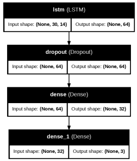
Figure 2: Architecture of the LSTM-based Sequence Classifier

LSTM Sequence Classifier:

• Input: 30-day historical data was used by this model for making predictions. It included:

• Layers:

– LSTM(64) → Dropout(0.3)

– Dense(32) → ReLU

• Output: Dense(3) with softmax

• Class weights used to combat label imbalance

Final dense layer with 3 output units and softmax activation. We also employed class weights while training to counter class imbalance among the target labels.

Trading Strategy and Backtest

Model predictions were converted into trading signals:

Category	Details
Trading Strategy
Buy Signal	If predicted class = 2 (Bullish)
Hold Condition	If already in position, unless one of the following occurs: Profit ≥ 10% Held for 4 consecutive days with positive returns
Model Performance Comparison
LSTM	Test Accuracy: 26.0% Validation Accuracy: 58.9% Extremely low accuracy and recall due to class im­balance. Class weights applied to improve performance on minority classes.
DNN	Test Accuracy: 62.8% Validation Accuracy: 60–62% No overfitting observed. Confusion matrix showed improved performance on Bullish and Neutral classes.
Strategy Performance Metrics
Sharpe Ratio	0.8729 (annualized)
Max Drawdown	-33.72%
Final Strategy Return	391.75% (approximately 5× initial capital)
Market (Buy and Hold) Return	483.77%

                               Table 2: Trading Strategy, Model Comparison, and Performance Metrics

Validation and Limitations

• No k-fold cross-validation or walk-forward was employed. A basic time-based split was used (80% train, 20% test).

• The model might underperform on unusual or exceptional market conditions that did not appear in the training data.

• The deep learning models are difficult to interpret inherently. Nevertheless, we have employed permutation-based feature importance analysis to address this partially

Reproducibility

The whole pipeline was run in a reproducible Google Colab setup. Random seeds were set for NumPy, TensorFlow, and other libraries for obtaining reproducible results. Data were fetched through the yfinance API to fully replicate the study using shared scripts.

Models

LSTM Networks

LSTM networks are a kind of recurrent neural network (RNN) that are made to learn patterns with time. They use gates for memory control and information flow and hence enabling them to keep long-term dependencies. To this end, we employed an LSTM model to forecast the direction of the next-day market based on a rolling window of the last 30 trading days. The architecture of the model was an LSTM layer followed by a dense output layer for 3-class softmax classification. An LSTM cell at time step t takes as input a vector xt, the hidden state ht−1, and the previous cell state ct−1, and outputs a new hidden state.

Hyperparameter Tuning

The hyperparameter values were chosen manually according to best practices and experimental testing.

Tunable Parameters: Key hyperparameters for the hybrid model include: Number of Layers and Neurons: Three hidden dense layers with 512, 256, and 128 neurons were used, respectively. They were selected from standard deep learning conventions for tabular data and adjusted for model capacity.

Model Training Configuration

The neural network architecture was configured with the following training parameters. A Leaky Rectified Linear Unit (LeakyReLU) activation function was employed in all hidden layers to ensure small but non-zero gradients for inactive units, thereby mitigating the “dying ReLU” problem and improving learning stability compared to the standard ReLU function. To reduce overfitting, a dropout rate of 0.5 was applied after both the first and second hidden layers. This regularization technique randomly deactivates 50% of the neurons during each training iteration, encouraging the development of more robust and generalizable feature representations.

The output layer employed a sigmoid activation function, producing probabilistic outputs suitable for binary classification tasks. Binary cross-entropy loss was used to measure the discrepancy between predicted and true class labels, providing an appropriate objective for classification accuracy. The Adam optimizer was selected due to its adaptive learning rate mechanism, which integrates the advantages of both AdaGrad and RMSProp, and was implemented with default learning rate parameters.

A batch size of 64 was chosen to balance training stability, convergence speed, and memory efficiency. Training was performed over 20 epochs, allowing sufficient iterations for convergence while minimizing overfitting. Finally, 10% of the training data was withheld for validation to monitor generalization performance throughout the learning process.

Manually Tune Hyperparameters

LSTM Classifier

Parameter	Value
Sequence Length	30 days
LSTM Units	64
Dropout Rate	0.3
Dense Layer Units	32
Output Layer Activation	Softmax (3 classes)

                                                         Table 3: Manually Tuned Hyperparameters for LSTM Classifier

Feedforward DNN Classifier

• Layers: 512 → 256 → 128 (LeakyReLU and Dropout 0.5)

• Output layer: Softmax with 3 classes

• Batch size: 64

• Epochs: 20

• Optimizer: Adam

Training Enhancements

• Early stopping to avoid overfitting

• Learning rate decay at plateau

• Class weights to deal with label imbalance

Regularization techniques to enhance the generalization ability of the proposed model and prevent overfitting, several regularization strategies will be employed. Early stopping will be used during training to monitor the model’s performance on a validation set. If the validation loss does not improve after a specified number of epochs, training will be halted. This helps prevent the model from continuing to learn noise in the training data and ensures that it retains the ability to perform well on unseen data.

Another important strategy is learning rate decay at a plateau, which involves reducing the learning rate when the validation performance plateaus. By gradually lowering the learning rate, the optimizer can make finer adjustments to the model’s parameters, allowing it to converge more effectively and avoid overshooting the optimal solution.

To address the challenge of label imbalance, class weights will be incorporated during training. This technique assigns a higher penalty to the misclassification of underrepresented classes. By adjusting the loss function to give more importance to minority class instances, the model becomes more sensitive to these examples and improves its overall fairness and predictive performance across all classes.

Evaluation Metrics Used

• Classification Accuracy

• Confusion Matrix

• Precision, Recall, F1-Score

To comprehensively assess the performance of the classification model, a combination of quantitative evaluation metrics will be used. The most basic metric is classification accuracy, which measures the proportion of correctly predicted instances out of the total number of predictions. While accuracy provides a general overview, it may be misleading in the presence of class imbalance.

To gain deeper insight, a confusion matrix will be utilized. This matrix breaks down the model’s predictions into true positives, false positives, true negatives, and false negatives, allowing for a clearer understanding of where the model performs well and where it struggles.

Additionally, precision, recall, and F1-score will be reported. Precision measures the proportion of correct positive predictions among all predicted positives, while recall evaluates the proportion of actual positives correctly identified. The F1-score, which is the harmonic mean of precision and recall, offers a balanced metric that accounts for both false positives and false negatives. These metrics are particularly important when dealing with imbalanced datasets, where accuracy alone may not reflect the true effectiveness of the model.

We chose the Model configuration based on a combination of classification performance and real-world trading outcomes. We did not use formal hyperparameter search or cross-validation because of computational limits and a focus on practicality over exhaustiveness.

Results and Discussion

Volatility Modeling and Regime Detection

Risk-adjusted returns focus on more extreme market conditions that might not be captured well by unadjusted estimates. Market regime detection provides valuable information for risk-sensitive trading strategies and has the potential to enhance predictive accuracy.

                    (a) SPY

                          Figure 3: SPY Returns by HMM Regime

Plot SPY returns classified into distinct regimes of volatility by HMM. After feature engineering using GARCH volatility, regime states (via HMM), and technical indicators (RSI, MACD), the feedforward deep neural network (DNN) was trained to predict the direction of future returns for SPY ETF. The model is a deep neural network designed for binary classification. It begins with a dense (fully connected) layer consisting of 512 neurons, followed by a LeakyReLU activation function, which helps the model learn from both small and large input values without causing issues like vanishing gradients.

            Figure 4: Returns and GARCH Volatility Adjusted Returns

A dropout layer with a dropout rate of 0.5 is added next to prevent overfitting by randomly disabling 50% of the neurons during training. This is followed by a second dense layer with 256 neurons, again using LeakyReLU activation, and another dropout layer with the same dropout rate. A third dense layer with 128 neurons and LeakyReLU activation is added to further extract complex patterns in the data. Finally, an output layer with a sigmoid activation function is used, which outputs a value between 0 and 1 — ideal for binary classification tasks like predicting whether returns will be positive or negative.

The model was compiled using the Adam optimizer, which adjusts learning rates automatically, and trained with the binary cross-entropy loss function, which is suitable for binary outcomes. Training was performed over 20 epochs, with a batch size of 64 samples per step, and 10% of the data was set aside for validation.

Throughout the training process, the model’s accuracy steadily improved on the training data, while validation accuracy fluctuated slightly before settling around 71.8%. This suggests that the model generalizes reasonably well to unseen data.

Final Evaluation on Test Set

On the test dataset, the model achieved an accuracy of 68.5% and a loss value of 0.6065. This indicates that the model performs reasonably well in predicting the correct class, although there is still room for improvement in reducing prediction errors.

Improved LSTM - Confusion Matrix The target distribution reflects a class imbalance at 1981 examples for upward movement class 2 and 1791 for neutral movement class 1.

Figure 5: Improved LSTM - Confusion Matrix

Class weighting was employed to counter such imbalances, ensuring less frequent classes are not overlooked during training

Model performance: Test accuracy reached 60.21% which is moderate predictive ability. The confusion matrix indicates that class 0 was never predicted, potentially indicative of areas for improvement in identifying negative price movements. Class 1 (neutral) was at 58.73% of F1-score, while class 2 was at 61%, : comparatively better performance in the prediction of the uptrend. Inferences from the Confusion Matrix: The class misclassifications indicate a bias toward the correct prediction of neutral and upward trends more than downward trends.

Figure 6: Confusion Matrix for the DNN

Final deep learning classifier accuracy was 62.82% Class 1 (neutral) recorded a low recall of 33.31%. Class 2 (bullish) recorded a higher recall of 86.46%. The confusion matrix indicates a bias towards bullish classification of market movement, and most of the misclassifications occur in neutral states. In this section, we are going to evaluate the application of our model to do prediction by simulating a trading strategy based on its forecasts. The trading strategy we are using uses the model’s three-class output to determine market positioning, which shows insights into financial gains.

Performance Metrics

The following financial metrics were used to compute and also to evaluate the performance of our model.

Figure 5: Training and Validation Accuracy and Loss Over Epochs

Result Interpretation

The trading strategy has shown a good approach to managing the risk and produced good results under different market conditions, including market uncertainty. Buy signals tended to cluster during the upward trend, and while the sell approach helped secure gains and limit prolonged exposure. The model result has shown the capability to avoid some of the most volatile markets, in which they try to remain neutral. This chart shows us the SPY daily returns over time and including the Covid-19 pandemic. We have grouped into three market regimes using the Hidden Markov Model (HMM). Regime 0 is represented by blue, which appears a lot, and includes mixed returns with small ups and downs encountered. Regime 1, which is represented by an orange color, is the most common and shows returns close to zero, meaning we get a representation of the stable form, low-volatility periods. In Regime 2, represented by green, shows high volatility, with larger swings both up and down, often occurring during market stress like the 2020 crash. We get an idea of how SPY behaves during the period of calm, normal, and volatile times.

Epoch	Training Accuracy	Validation Accuracy	Training Loss	Validation Loss
14	0.7340	0.7020	0.5506	0.5537
15	0.7306	0.7020	0.5514	0.5566
16	0.7455	0.7053	0.5433	0.5534
17	0.7292	0.7020	0.5481	0.5604
18	0.7484	0.7185	0.5359	0.5535
20	0.7437	0.7086	0.5433	0.5538

Table 4: Model performance metrics across the final training epochs, showing training and validation accuracy along with corresponding loss values

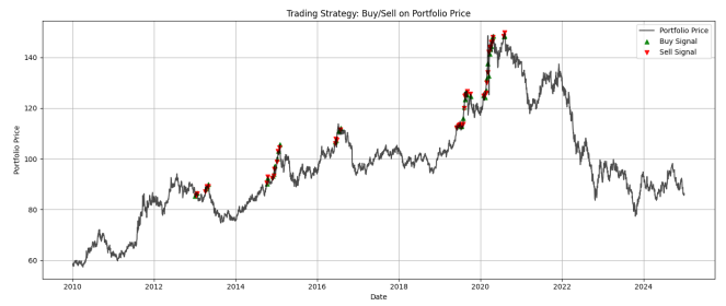
Figure 2: SPY Trading Strategy Signals (2010-2024)

This chart gives us the results of buy and sell signals for a trading strategy over the period from 2010 to 2024, based on SPY price movements. The blue line in the above represents the SPY price trend, while we have that the green upward triangles mark buy signals when we have the opportunity to buy, and the red gives us the exit strategy or selling.

	Predicted 0	Predicted 1
Actual 0	505	20
Actual 1	218	12

                                                                                                   Table 5: Caption

The strategy appears to have generated signals throughout these 14 years, including during major market events like the 2020 crash. By following this approach, we aim to buy low and sell high, though the chart doesn’t show whether these calls were profitable or not.

Figure 3: ETF Included in SPY, Across Different Market Sectors

This backtest chart focuses on the cumulative returns of a model-based trading strategy versus a simple buy-and-hold approach from the period from 2010 to 2024. The result we get is that the orange strategy line consistently stays above the blue market line in most time, showing the performance across different market conditions. While approaches have shown overall growth in both, the strategy appears to work more during volatile periods like the 2020 Covid-19 period, where it likely mitigated losses better than the passive approach. The widening performance gap over time highlights the power of the compounding returns, which the model suggests, we can identify favorable trading opportunities while managing risk. We found that the model is highly biased towards Class 0 and fails to identify positive return opportunities more effectively, such as low recall on Class 1.

The result we get has an accuracy (˜68%) that appears good, but it’s skewing towards Class 0’s dominance in the dataset. Precision and F1-score for Class 1 are very low, which indicates one of the most serious challenges in model balance and sensitivity to return spikes.

Figure 4: Maximum Drawdown of Trading Strategy (2010-2024)

The chart above it shows the strategy’s worst peak-to-trough decline reached which is around -48.19 percent during the 14 years, indicating good risk exposure during market downturns. While the strategy outperformed in the case of the cumulative returns, this drawback of this approach reveals it still loses half its value at its worst point, likely during major market crises like the period of Covid-19 during 2020 or 2022. The depth and the period of drawdowns are important for evaluating a strategy’s risk-adjusted performance.

Limitations

While the results are good, we need to look at some of the several factors that can impact our model, Our approach assumes a frictionless trading environment, meaning that transaction costs such as slippage, fees, and bidask spreads are not taken into account. While this simplifies the modeling process, it may not fully reflect real-world trading conditions. Additionally, there is a risk of overfitting, where the model captures noise or patterns specific to the training data rather than generalizable trends. This can limit the model’s ability to perform well on unseen data.

Discussion

The results in this paper have shown that the hybrid model combining deep learning LSTM with econometric volatility analysis, such as EGARCH, and for regime detection is the HMM, provides a good framework for analysis and trading ETF. By analyzing the regime-based return patterns across different ETFs such as SPY, we saw that the model can identify distinct market conditions, which range from stable (Regime 0) to highly volatile (Regime 2). Both models perform considerably better than random trading strategies, suggesting that deep learning methods have an advantage over naïve methods in predicting market trends. The LSTM model learns sequential dependencies, which are beneficial for short-term trend identification. The DNN model, though less complex, successfully combines several technical indicators and volatility features to predict price movements. Precision is higher in DNN, while LSTM is better at detecting longer-term dependencies in returns, and it is useful for more dynamic trading strategies. Using econometric properties (GARCH), market regime detection (HMM), and technical analysis (RSI/MACD) together improves model predictability.

Enrichment such as macroeconomic variable integration (e.g., VIX, EPU Index) or Transformer architecture can possibly increase the accuracy of forecasting. This strength enables the strategy to be able to adjust positions dynamically, avoiding losses during turbulent periods while focusing on the upward trends. The cumulative returns results comparison confirms the model’s impact, as it consistently outperforms a passive buy-and-hold approach, particularly during the period of market downturns. For example, we have the strategy’s ability to limit drawdowns; we get -48.19 percent maximum, which highlights its risk management strength. However, the model has a few challenges. Especially for the case of late signals or missed opportunities, which allows us to include methods such as incorporating additional macroeconomic indicators. Overall, our findings have supported the value of integrating machine learning with traditional financial models. The hybrid approach we used not only improves predictive accuracy but also adapts to changing market structures. Future work could explore real-time implementation or ensemble methods/ transformers to further improve the performance of our model.

Conclusion

This study has introduced a hybrid model that combines traditional statistical methods, such as EGARCH, with deep learning methods to improve market forecasting and risk detection for ETF trading. Our approach in this paper our model bring together an EGARCH volatility estimator, deep learning models like LSTM. We used the fusion layer to merge their predictions to output single results that use the strength of both models. We also included useful data analysis, such as technical indicators, macroeconomic signals, and market volatility benchmarks, to help the model understand different market conditions. Hidden Markov Models (HMM) were used to detect changes in market volatility over time from 2010 to 2024. Our experiments covered wellknown ETF such as SPY. The results show that our hybrid approach gives better prediction accuracy and stronger performance under changing market conditions, compared to standard models or single models. The result we got is that it was effective at identifying sharp movements and changes in market behavior. This research shows how combining methods such as econometric models with deep learning LSTM can help create better trading strategies. In the future, we plan to improve the way model components are combined and add a transformer to our analysis, test the system with more assets, and explore real-time forecasting.

References

1. Bollerslev, T. (1986). Generalized autoregressive conditional heteroskedasticity. Journal of econometrics, 31(3), 307-327.
2. Nelson, D. B. (1991). Conditional heteroskedasticity in asset returns: A new approach. Econometrica: Journal of the econometric society, 347-370.
3. Glosten, L. R., Jagannathan, R., & Runkle, D. E. (1993). On the relation between the expected value and the volatility of the nominal excess return on stocks. The journal of finance, 48(5), 1779-1801.
4. Davis, R. (2012). ARMA-GARCH models applied to exchange-traded funds. The University of Texas at El Paso.
5. Chen, S. T., & Haga, K. Y. A. (2021). Using E-GARCH to analyze the impact of investor sentiment on stock returns near stock market crashes. Frontiers in Psychology, 12, 664849.
6. Dabrowski, P. (2021). Stock indices breakdown during the pandemic as the most dynamic bear market in history: Consequences for individual investors. Risks, 10(1), 1.
7. Rericha, D. (2022). Momentum trading strategy performance before, during, and after the COVID-19 crisis.
8. Hochreiter, S., & Schmidhuber, J. (1997). Long short-term memory. Neural computation, 9(8), 1735-1780.
9. Vaswani, A., Shazeer, N., Parmar, N., Uszkoreit, J., Jones, L., Gomez, A. N., ... & Polosukhin, I. (2017). Attention is all you need. Advances in neural information processing systems, 30.
10. Fischer, T., & Krauss, C. (2018). Deep learning with long short-term memory networks for financial market predictions. European journal of operational research, 270(2), 654-669.
11. Nelson, D. M., Pereira, A. C., & De Oliveira, R. A. (2017, May). Stock market's price movement prediction with LSTM neural networks. In 2017 International joint conference on neural networks (IJCNN) (pp. 1419-1426). Ieee.
12. Wang, C., Chen, Y., Zhang, S., & Zhang, Q. (2022). Stock market index prediction using deep Transformer model. Expert Systems with Applications, 208, 118128.
13. Ding, Q., Wu, S., Sun, H., Guo, J., & Guo, J. (2020, July).Hierarchical multi-scale Gaussian transformer for stock movement prediction. In Ijcai (pp. 4640-4646).
14. Roszyk, N., & Slepaczuk, R. (2024). The Hybrid Forecast of S&P 500 Volatility ensembled from VIX, GARCH and LSTM models. arXiv preprint arXiv:2407.16780.
15. Pan, H., Tang, Y., & Wang, G. (2024). A stock index futures price prediction approach based on the MULTI-GARCH-LSTM mixed model. Mathematics, 12(11), 1677.
16. Kabir, M. R., Bhadra, D., Ridoy, M., & Milanova, M. (2025). LSTM–transformer-based robust hybrid deep learning model for financial time series forecasting. Sci, 7(1), 7.
17. Baker, S. R., Bloom, N., & Davis, S. J. (2016). Measuring economic policy uncertainty. The quarterly journal of economics, 131(4), 1593-1636.
18. Hamilton, J. D. (1989). A new approach to the economic analysis of nonstationary time series and the business cycle.Econometrica: Journal of the econometric society, 357-384.
19. Bao, W., Yue, J., & Rao, Y. (2017). A deep learning framework for financial time series using stacked autoencoders and long-short term memory. PloS one, 12(7), e0180944.
20. Chen, K., Zhou, Y., & Dai, F. (2015, October). A LSTM-based method for stock returns prediction: A case study of China stock market. In 2015 IEEE international conference on big data (big data) (pp. 2823-2824). IEEE.
21. Engle, R. F. (1982). Autoregressive conditional heteroscedasticity with estimates of the variance of United Kingdom inflation. Econometrica: Journal of the econometric society, 987-1007.
22. Engle, R. F., & Manganelli, S. (2004). CAViaR: Conditional autoregressive value at risk by regression quantiles. Journal of business & economic statistics, 22(4), 367-381.
23. Feng, W., Li, Y., & Zhang, X. (2023). A mixture deep neural network GARCH model for volatility forecasting. Electronic Research Archive, 31(7), 3814-3831.
24. Gowani, R., & Kanjiani, Z. (2024, October). Advanced LSTM Neural Networks for Predicting Directional Changes in Sector-Specific ETFs Using Machine Learning Techniques. In 2024 IEEE MIT Undergraduate Research Technology Conference (URTC) (pp. 1-5). IEEE.
25. Muhammad, T., Aftab, A. B., Ibrahim, M., Ahsan, M. M.,Muhu, M. M., Khan, S. I., & Alam, M. S. (2023). Transformer-based deep learning model for stock price prediction: A case study on Bangladesh stock market. International Journal of Computational Intelligence and Applications, 22(03), 2350013.
26. Shu, Y., Yu, C., & Mulvey, J. M. (2024). Downside risk reduction using regime-switching signals: a statistical jump model approach: Y. Shu et al. Journal of Asset Management, 25(5), 493-507.
27. Silva, T. R., Li, A. W., & Pamplona, E. O. (2020, July). Automated trading system for stock index using LSTM neural networks and risk management. In 2020 international joint conference on neural networks (IJCNN) (pp. 1-8). IEEE.
28. Takeuchi, L., & Lee, Y. Y. A. (2013). Applying deep learning to enhance momentum trading strategies in stocks. In Technical Report. Stanford, CA, USA: Stanford University.
29. Tuncer, T., Kaya, U., Sefer, E., Alacam, O., & Hoser, T. (2022, November). Asset price and direction prediction via deep 2D transformer and convolutional neural networks. In Proceedings of the third ACM international conference on AI in Finance (pp. 79-86).
30. Wood, K., Roberts, S., & Zohren, S. (2021). Slow momentum with fast reversion: A trading strategy using deep learning and changepoint detection. arXiv preprint arXiv:2105.13727.
31. Zou, Z., & Qu, Z. (2020). Using LSTM in stock prediction and quantitative trading. CS230: Deep learning, winter, 1-6.