Corn to Ethanol: Design, Simulate and Statistical Optimization for Sustainable Biofuel Production

Introduction

In the pursuit of sustainable energy solutions, the design and optimization of corn-to-ethanol plants play a vital role in the United States, a leader in biofuel production. Corn ethanol, a widely utilized renewable fuel, is produced through a multi-step process that involves milling, fermentation, distillation, and dehydration. The efficiency and productivity of these plants are critical for maximizing ethanol yield while minimizing environmental impact. Optimizing the design of such facilities involves balancing various factors, such as raw material input, energy consumption, and waste management. With the USA contributing significantly to the global biofuel market. The country produced approximately 15.8 billion gallons of ethanol annually, with corn being the primary feedstock. As advancements in technology continue, the ongoing pursuit of innovative plant designs and optimization strategies is essential to enhance the sustainability and competitiveness of corn-to-ethanol production in the United States. Ethanol, when used as a fuel, offers specific environmental benefits over fossil fuels due to its cleaner burning properties. It significantly reduces greenhouse gas emissions, cutting carbon dioxide emissions by about 34% compared to gasoline, according to the U.S. Department of Energy. Additionally, ethanol is produced from biomass, which absorbs CO2 as it grows, contributing to a further reduction in net greenhouse gas emissions. A study by Vörösmarty et al. (2022) explores the spatial distribution of potential bioethanol yield from corn and other bioenergy crops across the U.S., considering environmental impacts like drought and heat on yield. This comprehensive analysis uses the Integrated Science Assessment Model (ISAM) for its calculations with bioethanol yield and sustainability [49]. Irwin's analysis from the University of Illinois at Urbana-Champaign discusses the profitability of ethanol production in 2023, highlighting factors that contributed to strong profits despite market volatilities. Recent research focuses on the sustainability of producing bioethanol from grain and tuber starch feedstocks and different pretreatment strategies for optimizing bioethanol production [51-52].

Ethanol (C2H5OH), also known as ethyl alcohol, is an organic chemical most known for its use as a fuel additive and beverage. At ambient temperatures and pressures, it is a clear, colorless, and volatile liquid. It has a relatively low freezing point (-114° C), low boiling point (78° C), and low density (0.789 g/mL) liquid [4]. Usually ethanol and water are commonly very miscible due to their similar intermolecular interactions. Both molecules contain hydroxyl (-OH) groups which increase polarity and allow for hydrogen bonding [5]. The hydroxyl group serves as a reactive site in organic reactions such as dehydration, dehydrogenation and esterification for ethanol. Ethanol can be used to form common industrial chemical feedstocks such as ethylene and acetaldehyde. Therefore, pure ethanol should be handled separately from other reactive organic compound to avoid unnecessary byproducts.

Ethanolis high flammable with a flash point 14° C. Vapor concentrations of ethanol as low as 3.3% by volume are potentially explosive [5]. To avoid risk of explosion, it should be stored at lower temperatures and kept away from any source of ignition. Although ethanol vapors are typically not toxic, liquid doses as low as 75–80 g can cause intoxication and 250–500 g can be fatal [5]. It should therefore be consumed sparingly and in low doses.

Table-1 compares ethanol with other biofuels (biodiesel, butanol, and methanol) across several important properties: energy content, octane number, CO2 emissions reduction, production cost, and water solubility. These properties highlight the significance of ethanol as a sustainable and eco-friendly biofuel option.

underground storage system storing fuels with over 10% ethanol (E10), under CFR 280.32. This includes tanks, piping, and spill and overfill equipment, ensuring all components can safely store the specified ethanol blends [43]. This focus on safety and regulatory compliance in handling ethanol is crucial for enhancing the corn-to-ethanol production process, reinforcing the commitment to sustainable practices and the safe production of biofuels.

Historical Use of Ethanol

Ethanol has been used for centuries, initially in beverages and later as a fuel. The first significant leap in production technology occurred in the 19th century with thedevelopment of the distillation process, allowing for more efficient ethanol production. By the early 20th century, Henry Ford designed his Model T to run on ethanol, highlighting its potential as a renewable fuel source. In recent years, the United States has become a leading producer of ethanol, with production reaching over 15 billion gallons in 2020 (U.S. Energy Information Administration, 2021). This growth is largely due to advancements in fermentation technology and the use of genetically modified yeasts, which have increased yield and efficiency. Today, ethanol is not only a biofuel but also used in pharmaceuticals and cosmetics, demonstrating its versatile application across industries.There are different grades of ethanol based on the usage. The grades depend on water content, alcohol content, impurity profile, production standard and denaturant type. Ethanol has three major purposes to be used: fuel ethanol, beverage ethanol, and industrial ethanol. Table-2 states the different grade of ethanol along with their purity [26].

                                                          Table 2: Different graded ethanol and respective usage [26]

Fuel ethanol, a vital component in the realm of motor fuels, is intricately interwoven with gasoline to bolster its efficacy. Meanwhile, beverage ethanol is harnessed for the synthesis of potable libations, while industrial ethanol serves as a vital chemical precursor, predominantly employed in the manufacture of pharmaceuticals and polymers [6]. The strategic promotion of ethanol during the Second World War by the US Government marked its inaugural foray into the augmentation of the national transportation fuel supply [27]. Noteworthy historical benchmarks include the production of approximately 175 million gallons of ethanol in the USA by 1980, a milestone that has since undergone significant transformation. The year 2005 witnessed the enactment of the Energy Policy Act, heralding a renewable fuel standard escalation from 4 billion gallons in 2005 to 7.5 billion gallons in 2012. This legislative impetus precipitated heightened ethanol plant construction and intensified scrutiny of diverse feedstocks, including corn, grass, and trees. The denouement of 2006 witnessed a monumental

achievement as fuel ethanol consumption in the United States soared to 4.9 billion gallons, surpassing the 4.2-billion-gallon mandate stipulated in the Energy Policy Act. Presently, the US ethanol landscape is dominated by fuel ethanol, constituting 92% of its utilization, with 4% allocated to beverages and an additional 4% earmarked for diverse industrial applications [16]. The widespread integration of ethanol, notably with over 95% of US gasoline infused with this biofuel, underscores its vital role in augmenting octane levels and displacing more environmentally deleterious additives such as methyl tertiary butyl ether (MTBE). Functioning as an oxygenating agent in gasoline blends, ethanol enhances combustion efficiency, mitigating carbon monoxide emissions, a salient facet in curtailing the deleterious byproducts of incomplete combustion [8]. This multifaceted utility has engendered global resonance, rendering ethanol a ubiquitous and indispensable component in the contemporary fuel landscape. The ensuing figure-1 encapsulates the trajectory of fuel ethanol production among major nations, with a focus on the year 2016.

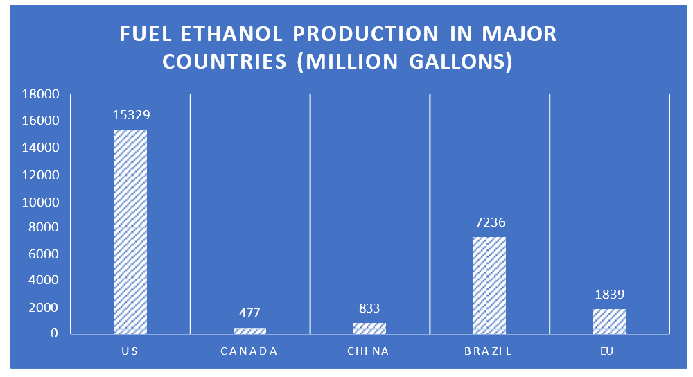
Figure 1: Fuel ethanol production (million Gallons) by major countries [33]

The total US fuel production in 2016 was 15.3 billion gallons which is around 60% compared to the ethanol production of other major countries. [33]. Second highest ethanol producing country is Brazil [33]. Corn-derived ethanol is primarily used in the fuel industry, where it serves as a renewable biofuel and an oxygenate additive to gasoline, enhancing combustion and reducing emissions. The ethanol fuel blends, such as E10 (10% ethanol and 90% gasoline) and E85 (85% ethanol for flex-fuel vehicles) proves corn ethanol's role in diversifying energy sources. Beyond the automotive sector, corn ethanol finds applications in the production of beverages and industrial solvents, benefiting from its high purity and renewable origin. The versatility of corn-derived ethanol, supported by the efficiency of conversion from starch to ethanol, underscores its significance in the transition towards cleaner energy and sustainable industrial practices. The diverse applications and significance of ethanol across various industries are fundamentally influenced by its purity and grade. Table-3 states the specific grades of ethanol, their respective applications, purity requirements, and the implications of these standards on their suitability for different applications.

                                       Table 3: Applications and Purity Requirements of Ethanol Across Various Industries [44-45]

History of Corn-Ethanol Industry industry

In 1999, an estimated 1.48 billion gallons of fuel ethanol were blended with gasoline for use in motor vehicles [1]. The predominant feedstock for ethanol production in the United States is shelled corn, processed through either wet milling or dry milling techniques. Wet milling, characterized by higher production efficiency and capital intensity, yields corn oil, animal feed products, and starch-based commodities such as ethanol, corn syrups, or cornstarch. Approximately 60% of ethanol production emanates from wet milling facilities [2]. Conversely, the dry milling process, which emerged in 1970 due to a reliance on alternative energy sources amid an oil embargo, primarily yields ethanol and dried distillers' grains (DDG), a valuable animal feed byproduct. Both processes yield carbon dioxide (CO2), with some facilities capturing and commercializing this emission. Notably, the cost-effectiveness of the dry milling process facilitated a decrease in ethanol production costs, with the estimated price per gallon at approximately $2.47 in 1978

[3]. The year 2013 witnessed the sale of over 13.3 billion gallons of ethanol, valued at approximately $2.50 per gallon, contributing to a total industry worth of $33 billion [28, 29]. The proliferation of US ethanol production from less than 2 billion to over 13 billion gallons annually between 2000 and 2015 was catalyzed by the introduction of the E 10 fuel blend (10% ethanol content), aligning with vehicle design specifications. The current fleet comprises around 15 million flexible fuel vehicles, with a projected increase, capable of utilizing this blend, and an expanding market for E 85 fuel [18]. Ethanol production facilities exhibit varying capacities, ranging from 1 or 2 million gallons to several hundred million gallons per year. While larger facilities benefit from economies of scale, other considerations, such as proximity to corn growers to mitigate shipping costs and the utilization of wet co-products as animal feed to reduce drying expenses, contribute to the overall cost dynamics [18]. The intricate relationship between US corn production and its allocation for fuel purposes is illustrated in Figure 2. [34].

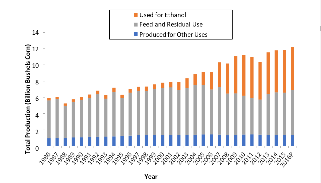
Figure 2: US corn production and usage for fuel [34].

The overall trend shows increasing production. Corn production for ethanol usage increased from 2001 to 2010. The increased ethanol seems to have come from the increase in overall corn production [34].

Environmental Impacts of Ethanol

Ethanol fuel presents a noteworthy environmental benchmark relative to conventional gasoline, primarily attributable to its role as an oxygenating agent that enhances combustion performance, thereby mitigating carbon monoxide emissions [9]. Legislative amendments to the Clean Air Act in 1992 mandated reductions in carbon monoxide emissions, marking a vital stride toward cleaner-burning fuels [10]. However, the early 2000s revealed concerns regarding the contamination of groundwater and associated public health risks arising from the use of methyl tertiary-butyl ether (MTBE) [10]. Ethanol emerged

as an environmentally sound energy solution, serving as a fuel additive that avoids air and water contamination. It is essential to acknowledge, however, that ethanol production facilities are not devoid of environmental impact, as they release acetaldehyde—a potential carcinogen—and contribute to emissions of nitrogen oxides (NOx) and volatile organic compounds (VOCs), akin to traditional gasoline [10]. Notably, the overarching concern for the greenhouse effect and climate change stems from carbon dioxide emissions resulting from the combustion of fossil fuels [10]. In contrast, ethanol, being a biofuel derived from biomass, facilitates a carbon cycle wherein carbon is exchanged between the atmosphere and the corn crop, ensuring a consistent overall carbon concentration. Corn, owing to its ubiquity and ease of production in the United States, predominates as the principal source of ethanol [11].

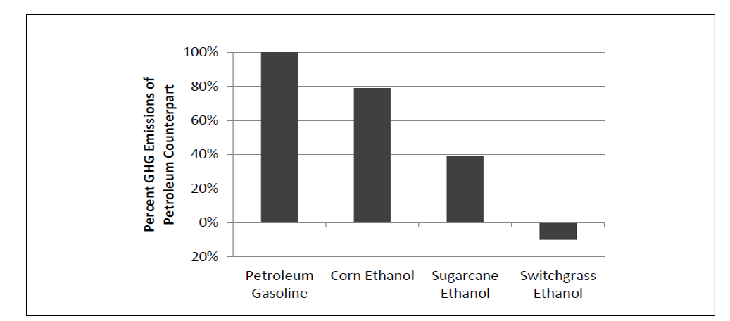
 Figure 3: Lifecycle greenhouse gas Emissions from Biofuels, Compared to Petroleum Substitutes [12] 

It can be seen here that corn ethanol, despite its popularity, only reduces carbon emissions by 21%. Switch-grass ethanol is a very effective alternative, reducing carbon emissions by an incredible 110% due to its ability to trap carbon within the soil and its biomass. Ethanol can also be produced from cellulose which is a good alternative of corn to ethanol. This has the added benefit of leaving the corn kernel for use as food when compared to typical corn ethanol which uses the entire plant. Although cellulosic ethanol is not commonly used due to a more complex and expensive fermentation process, it should not be ignored as a potential source for ethanol in the future.

The environmental impacts and sustainability considerations of ethanol production, especially from corn, are indeed critical aspects to evaluate when discussing the long-term viability of ethanol as a renewable fuel source. A study published in the Proceedings of the National Academy of Sciences highlights that ethanol could be at least 24% more carbon-intensive than gasoline. The increase in corn cultivation for ethanol production may lead to a significant expansion of cropland, resulting in carbon release from soil tilling and emissions from farming activities, such as the use of nitrogen fertilizers [46]. Furthermore, the economic and environmental implications of ethanol production are intertwined with the prices of corn and oil, affecting food supply and prices. As ethanol production surged, it may lead to higher corn prices, impacting food and feed prices globally. Ethanol's profitability and environmental efficiency are influenced because higher corn prices make ethanol more expensive and less competitive compared to oil. These dynamic underscores the complex trade-offs between

using corn for fuel versus food and the broader environmental impacts, including land use changes and water usage [47]. Water usage is another critical environmental concern. Corn cultivation for ethanol requires substantial amounts of water for irrigation, contributing to water scarcity in some regions. The National Renewable Energy Laboratory (NREL) suggests that the water footprint of corn ethanol can significantly vary based on cultivation practices, with irrigated corn requiring much more water than rainfed corn [48]. While ethanol production from corn is promoted as a renewable energy source, its environmental and socioeconomic impacts present significant challenges. The sustainability of ethanol as a renewable fuel source needs to be critically evaluated in the context of its full lifecycle emissions, including the effects of land use change, water usage, and its implications for food prices and security. Future research and policy development should aim to mitigate these impacts through improved agricultural practices, efficient water use, and balanced energy policies that consider the complex interplay between energy production, environmental sustainability, and food security.

Energy Consumption in Different Corn-Ethanol Process Plants

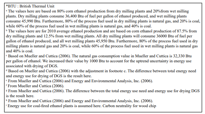
The level of energy consumption and greenhouse gas emission differs from type to type ethanol plants depending on the process fuel. The process fuel includes natural gas, coal, chips and so on. The following table 4 and the footnotes are adapted from literature to show the level of energy consumed in different process fuel driven ethanol plants [27].

              Table 4: Energy use in different types of ethanol plant (per gallon ethanol produced) [27] 

The corn-to-ethanol sector in the United States plays a vital role in the biofuel landscape, contributing significantly to the economy and the renewable energy. In 2022, the industry not only supported over 78,800 direct jobs but also had a broader economic impact, creating $34.8 billion in household income and contributing just over $57 billion to the nation's GDP. These figures underscore the sector's importance, marking the second-highest GDP contribution ever recorded. The industry also spent nearly $47 billion on raw materials and other inputs, with corn purchases alone accounting for more than $38 billion, highlighting the critical link between ethanol production and agricultural markets [38]. However, the industry faces several challenges, particularly in operational efficiency and market dynamics. The U.S. ethanol market entered 2023 amidst concerns of overproduction relative to demand, a situation exacerbated by falling winter temperatures and reduced driving demand due to high gas prices. Ethanol plants had to choose between continuing production at a loss or shutting down, risking even greater financial fallout. Despite these challenges, ethanol production remained above 1 million barrels per day for the last nine weeks of 2022, signaling resilience in the face of adverse conditions

[39] Operational efficiency has seen trends of improvement over the years, with ethanol conversion rates from corn and sorghum feedstock showing an upward trend from 2014 to 2019, achieving a peak near 3.00 gallons per bushel. This reflects a roughly 9 percent total increase in efficiency or about a 1.8 percent gain per year. Despite a dip during the coronavirus pandemic, the rate recovered to 2.97 gallons per bushel by September 2021, although no significant growth in conversion rates has been observed since mid-2019. This stagnation highlights the need for technological advancements and efficiency improvements in the sector [40]. Incorporating recent technological advancements, policy and economic impacts, sustainability metrics, market trends, and feedstock diversification into a unified narrative, the corn-to-ethanol industry is evolving rapidly. Innovations such

as advanced fermentation processes and genetically engineered yeast strains are enhancing efficiency and yields. Adjustments in the Renewable Fuel Standard and biofuel tax incentives are critically influencing the sector's competitiveness. Updated lifecycle analyses reveal corn ethanol's improved greenhouse gas emissions, water use, and energy return on investment compared to other biofuels and fossil fuels. Meanwhile, shifts toward electric vehicles and international ethanol demand trends underscore the dynamic market environment. Additionally, research into cellulosic and alternative feedstocks is promising to mitigate food crop competition and bolster sustainability, marking a significant stride towards a more adaptable and environmentally conscious ethanol production landscape.

Material and methods

Ethanol is produced from corn through the fermentation process. In a fermentation process, microorganisms called yeast are used to metabolically convert sugars into ethanol and carbon dioxide via the simplified chemical reaction below [19].

C₆H₁₂O₆ 2C₂H₅OH + 2 CO₂

Fermentation is a complex process that requires a good deal of preparation before exposing the corn feed to the yeast. Additionally, there are several valuable products and byproducts that must be purified and separated after fermentation has taken place. Ethanol plants typically carry this preparation and purification out through one of two major processes: dry grind and wet mill. The steps involved in each of these processes are outlined in following Figure 4. The entire mash is fermented into dry milling where only starch is fermented in wet milling. The starch is then cooked, or liquefied, and an enzyme added to hydrolyze, or segment, the long starch chains. In dry milling, the mash is cooked and an enzyme added. In both cases a common enzyme is added to convert the starch into sugar and glucose

through saccharification [32]. In wet milling, the saccharification take 48 hours or less depending on the enzyme and in dry milling, saccharification has been combined with the fermentation step in a process called simultaneous saccharification and fermentation (SSF). Glucose is then fermented into ethanol by yeast. The mash must be cooled to at least 95° F before the yeast is added. The yeast converts the glucose into ethanol, carbon dioxide (CO2), and small quantities of other organic compounds during the fermentation process. The yeast produces almost as much CO2 as ethanol, ceases fermenting when the concentration of alcohol is between 12 and 18% by volume, with the average being about 15%. The process is accompanied with a distillation step to separate the ethanol from the alcohol-water solution. Usually

the separation involves two steps; distillation and dehydration. Primary distillation yields ethanol that is up to around 90% EtOH. Dehydration further increases the purity of ethanol. Dry milling production leaves, in addition to ethanol, distiller’s dried grains with solubles (DDGS). The feed co-products must be concentrated in large evaporators and then dried. The CO2 may or may not be captured and sold. Due to the greater simplicity of the dry grind process, dry mill is significantly more common and is utilized in approximately 75% of all ethanol production processes [14,15]. While dry-milling plants have higher yields of ethanol; the wet mill is more versatile because the starch stream, being nearly pure, can be converted into other products.

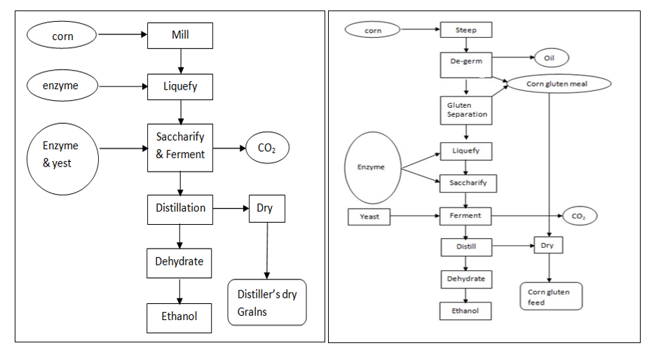
Figure 4: Comparison of ethanol formation process [18] DRY GRIND & WET MILL

Both processes involved cleaning of the corn prior to entry into the mill. In the dry mill process, the corn is grained and water is added to form mash. Wet mill has more steps compare to dry mill. Unlike the dry mill process, the components are separated from the grain. The corn is treated a dilute acid treatment where it is steeped into a solution of water and sulfur di oxide (SO2). In the wet mill, milling and processing are more elaborate because the grain must be separated into its components. Therefore, in wet milling, the construction cost is higher due to the need of constructing additional tanks for soaking 30-40 hrs. Then the

kernel is separated from the germ and corn oil is extracted from the germ. The co-products are corn oil, Corn Gluten Feed (CGF), Corn gluten meal (CGM) and others [31].

Generic Simulation of a Corn-Ethanol Plant

A steady state simulation is essential to understand the process, environmental and business ramifications of different configurations. PRO/II has been used to model the bioethanol process. The conversion reactor and a calculator unit operation provide customization for glucose fermentation.

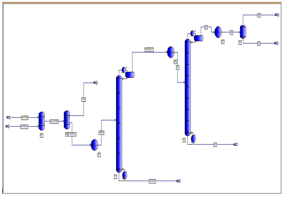
Figure 5: PRO/II simulation of corn-ethanol plant [20] 

The simulation has been done with the following objectives [20]:

• Analyze cause and effect.

• Justification for process improvement

• Picture of process outcome at different conditions

• Optimize bioprocess.

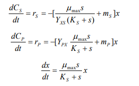
The conversion rate from starch to glucose and glucose to ethanol was determined based on the following journal article: “Parameter Estimation for Simultaneous Saccharification and Fermentation of Food Waste into Ethanol Using Matlab Simulink” by Rebecca Anne Davis. The conversion rate is based on 90 g/l of starch that produces 80 g/l of glucose. Finally 92 wt% ethanol was achieved. The rate equations for this process are given below [20]:

Ethanol was produced from starch content in corn via forming glucose as an intermediate product. The data for the conversion was simulated using PRO/II and then the separation scheme was established for getting greater than 90 wtâ?? ethanol. To simulate the hydrolysis reaction, water and starch from corn were fed in the reactor at pressure of 14.7 psi and temperature of 25° C at the molar flow rates of 1000 kgmol/hr and 1 kgmol/hr respectively. The temperature of the conversion reactor was maintained at 180° C and zero pressure drops was assumed. NRTL thermodynamic model was used system. Hydrolysis reaction produced 86 wt% glucose and 9 wt% unconverted starch where the molar flow rate of glucose and starch were 712 kgmol/hr and 0.11 kgmol/ hr. The outlet stream of hydrolysis reactor was fed to the second conversion reactor at temperature of 35° C and pressure of 14.7

Assumptions Made to Generate a Process Model

• Steady state

• Starch is composed of 800 glucose units.

• The unconverted components were considered insignificant as product streams.

Ethanol was produced from starch content in corn via forming glucose as an intermediate product. The data for the conversion was simulated using PRO/II and then the separation scheme was established for getting greater than 90 wtâ?? ethanol. To simulate the hydrolysis reaction, water and starch from corn were fed in the reactor at pressure of 14.7 psi and temperature of 25° C at the molar flow rates of 1000 kgmol/hr and 1 kgmol/hr respectively. The temperature of the conversion reactor was maintained at 180° C and zero pressure drops was assumed. NRTL thermodynamic model was used system. Hydrolysis reaction produced 86 wt% glucose and 9 wt% unconverted starch where the molar flow rate of glucose and starch were 712 kgmol/hr and 0.11 kgmol/ hr. The outlet stream of hydrolysis reactor was fed to the second conversion reactor at temperature of 35° C and pressure of 14.7psi. This reactor converts the glucose into ethanol and carbon dioxide. Carbon dioxide leaves the reactor as vapor phase at 960 kgmol/hr from the top outlet of conversion reactor. The top outlet stream also contains negligible amount of ethanol and glucose. The bottom outlet stream leaves at a flow rate of 1388 kgmol/ hr which contains 880 Kgmol/hr ethanol along with negligible amounts of starch, glucose, water and CO2 . This bottom stream is fed to a heat exchanger to get heated up from 35° C to 47° C, which acts as a pre heater for the distillation column. The outlet stream of the heat exchanger is fed to distillation column having 8 equilibrium trays, a condenser, a reboiler and operating at a reflux ratio of 3. The fourth tray was taken as the feed tray location and the parameters were found by using a short cut column. The ethanol rich product stream was recovered in vapor phase at temperature of 96° C with the discharge from the bottom as liquid phase. The molar flowrate of overhead product and bottom waste are 1188 kgmol/hr and 200 kgmol/ hr respectively. The top stream of distillation tower is 74 wt% ethanol. Product from this distillation tower was in vapor phase and we did not condense it except for the reflux stream because it mainly consisted of volatile matters and will require a lot of energy. To prepare a semi vaporized feed for next distillation tower a heat exchanger was used. Outlet stream was cooled down from 96° C to 78° C (higher than dew point of ethanol). The stream was fed to a distillation column with 10 equilibrium trays, a condenser, a reboiler, and operating at a reflux ratio of 1. As a simulation parameter we specified the bottom removal rate 6000 kg/hr. Feed was given at 5th tray of a distillation column. The purpose of this column is to achieve 90 wt% ethanol. The molar flow rate of the overhead product of second distillation tower was 1085 kgmol/hr and it was at temperature of 77C and it contained 89 wt^c\o ethanol along with 8 wt% water and some CO2 . This CO2 content had to be removed to achieve the desired purity. Hence the stream was cooled down to temperature of 65° C through a heat exchanger. At temperature of 65C ethanol and water condensed and a flash drum was used to separate out CO2 and at the bottom of flash drum desired 92 wt^c\o ethanol was achieved at a molar flow rate of 813 kgmol/hr where the entire bottom stream molar flow rate was 1007 kgmol/hr.

Reproduction of the Fermentation Optimization of Corn to Ethanol Process Using RSM

The statistical tool that was used for this optimization is called response surface methodology (RSM). RSM explores the interaction of different variables that affect the process response. The method was introduced by George E. P. Box and K. B. Wilson in 1951. This method uses a sequence of design of experiments to obtain an optimum response. Usually, RSM is used to maximize the production of a special substance by optimization of operating factors. Unlike the conventional trial and error method, RSM used a statistical technique to find the interaction among the variables. Response Surface Methodology (RSM) is applied only after completing the initial phases of experimentation that include: two-level fractional factorial designs that screen the vital few from the trivial many factors and then full-factorial designs that study the vital few factors in depth and define the region of interest. The goal of RSM is to generate a map of response, either in the form of contours or as a 3D rendering. While the system is more complicated, center composite design (CCD) can be implemented to estimate a second-degree polynomial model, which is still only an approximation at best.

Fermentation is the key step of corn to ethanol conversion for both dry and wet process. It is a chemical process through which bacteria metabolize sugar to alcohol. Corn contains starch which is the primary feedstock for fermentation. During the fermentation process, the generation of heat plays an important role because it increases the temperature. Also, the yest is exposed to different environments related to temperature change, stress, bacterial contamination and concentration. Also due to ethanol conversion, the growth rate of yest get inhibited and consequently slow down. pH of the medium also significantly influence the fermentation output. Therefore, better monitoring of fermentation process can significantly increase the ethanol production. [37]. A previous literature will be studied here to reproduce the optimization condition using Design-Expert software [21]. Along with the outcome of previous literature, new analysis will be performed to check the validity of statistical model. The key process variables were taken as pH, temperature, and substrate concentration for fermentation. This study will further analyze the statistical data distribution and transformation to check the model validity. Experimental setup for optimization process consist of Central Composite design which was applied to the experimental data of variables. Three batches were arranged while each batch contains two variables with one constant parameter. Each batch has nine runs. The high level and low level of all variable were obtained from literature [21].

Result and Discussion

Simulation Data Analysis The following table 5 shows the mass% of ethanol after two steps distillation and followed by flash tower.

                                                         Table 5: Mass composition of the Final product stream

From the simulation result of proposed model, the final product stream is obtained in liquid form with total molar rate of 1007.74 kgmol/hr and total mass rate of 41012.88 kg/hr. The stream leaves at 72° C temperature and atmospheric pressure. Specific enthalpy is 46.57 kcal for per kg of product. The mole fraction of ethanol into the product stream is 80% and water is 19% with minor quantities of unconverted substances.

                                       Table 6: Stream properties of the important streams of the design

Optimization Data Analysis

Optimization by Varying Temperature and pH

                                        Table 7: The combined effect of pH and temperature on ethanol production [21]

• Model equation generated by software:

Y = +76.40 − 7.85A−1.25B − 0.57AB −13.78A² −12.95B²

Where, A=Temperature, B=pH, Y=Ethanol concentration

• Analysis of variance of model -1 (pH and temp.):

                                                  Table 8: Analysis of variance of quadric model 1[21]     

 We know while the Fcalculated value of any model becomes larger than Fcritical value, the model became significant. A significant model means the equation and terms that are generated by software is also important. Here the F value of the model is 310.89 which imply the significance of the model. Furthermore, the P value shows the probable chance of noise in the model. While the P value is less than 0.05, it means the model is very unlikely affected by noise. If the P value becomes more than 0.1, the model or the terms are no more significant. The ANOVA table reveals a statistically significant model for predicting ethanol production, underscored by an F-value of 310.89 and a p-value of 0.0036, indicating robust model significance. Individual terms, such as pH (F-value: 283.15, p-value: 0.0016) and temperature squared (F-value: 669.71, p-value: 0.0016), demonstrate significant effects on ethanol production, affirming their relevance. Conversely, the interaction term AB shows no significant effect (p-value: 0.4125), suggesting minimal interaction between pH and temperature. The Adequate Precision ratio of 43.110 suggests an excellent signal-to-noise ratio, further validating the model's predictive capability and emphasizing its practical utility in optimizing ethanol production conditions. Therefore, the effect of pH and temperature are significant on ethanol production. Furthermore the ‘Diagnostics’ tab will be checked by design expert software to confirm the model validation.

Statistical Distribution and Transformation Analysis for pH-Temperature Model

In statistics, Design of Experiment (DOE) has a set of certain objectives. Firstly is to determine the statistical validity of the experimental result. Secondly is to reduce the number of experimental runs. Thirdly is to determine the significant factors which have most influence on the process outcome. DOE identifies the remaining insignificant factors which will contribute to the residual and lumped into error. The rule of the validating an experimental result is that the residual should have the normal distribution which means they should fall into a line and they must not have any specific pattern or shape (mostly a big fat S shape). Because the regular behave of the error is that 50% of the errors are less than zero while the other 50% are more than zero. If the errors are non-normal, the plot may be a curve. Therefore the normal probability plot of residual is a graphical tool to understand the normality of the model.

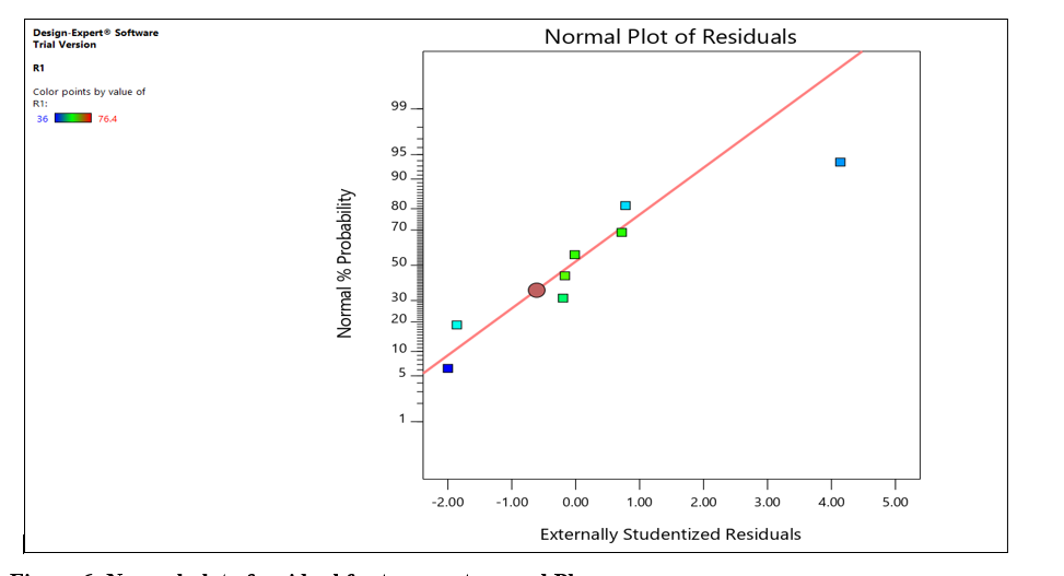
Figure 6: Normal plot of residual for temperature and Ph

Here it seems there are no S shape curve generated and all the data close to a straight line. It means the residual are normally distributed.

The other recommended diagnostic plot is the residual vs predicted response. Ideally the vertical spread of data is approximately same from left to right (assuming the constant variance). But while the residual vs predicted data follow a megaphone pattern (<), it means residual is also increasing with the predicted level.

Figure-7 shows no megaphone pattern appear in the residual vs predicted plot. It means their spread (variance) for different predicted values are constant. Therefore, the model is appropriate, and no transformation needed.

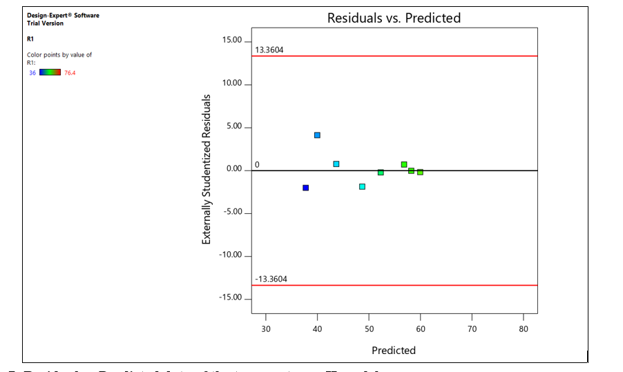
Figure 7: Residual vs Predicted data of the temperature-pH model. 

Contour Plot for temperature-pH model

As the model is found significant, the interference between pH and temperature can be drawn from the following 3D contour plot

which is generated by the software

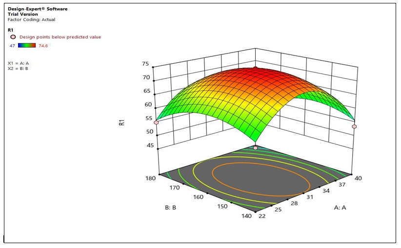
Figure 8: Contour plot showing the effect of pH and temperature on ethanol production. 

The figure8 shows the curvature which implies the importance of quadric equation. So the equation involves A2 and B2 are rightly selected. If the relationship will be linear, only a flat surface would appear. This curvature can be rotated to get different amount of ethanol production while changing the pH and temperature. Also, the effect of pH is more significant than temperature due to lower P value. The software will also generate the numeric solution of the optimization. Numeric solution of optimization for pH-temperature model is stated at figure -9.

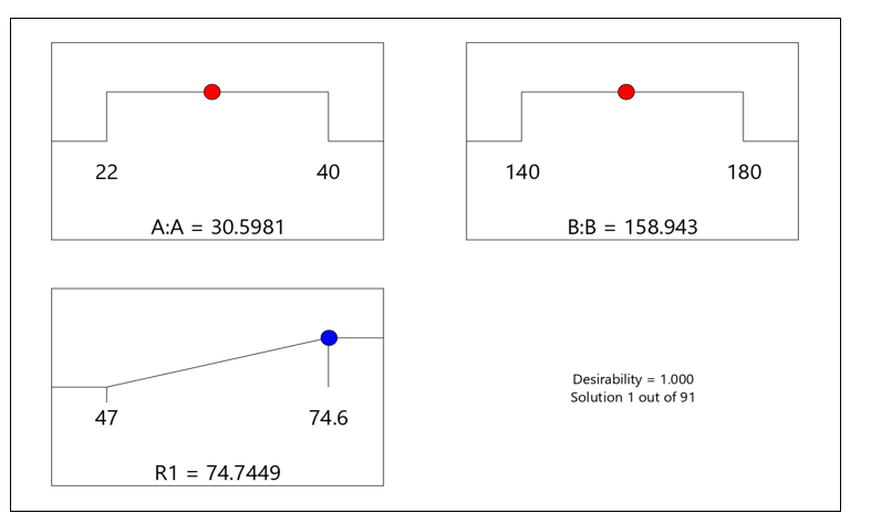
Figure 9: Optimization of pH and temperature for maximizing the ethanol concentration 

Optimization by Varying Temperature and Substrate Concentration

Table 9: The combined effect of temperature and substrate concentration on ethanol production [21] Model equation generated by software:

Y = +74.60 −1.95A−1.92B − 0.37AB −13.33A2 − 5.83B2 Where, A=Temperature, B=Substrate concentration,Y=Ethanol concentration

 Analysis of variance of model-2 (Temp. and substrate concentration)

                                           Table 10: Analysis of variance (ANOVA) of quadric model 2 [21]

The ANOVA table demonstrates a significant model for evaluating the effects of temperature and substrate concentration on the response variable, indicated by an F-value of 89.23 and a p-value of 0.0021, asserting the model's statistical significance. The quadratic terms of temperature (F-value: 389.73, p-value: 0.0036) and substrate concentration (F-value: 74.57, p-value: 0.0054) are notably significant, highlighting the critical influence of these factors' interactions on the outcome. The Adequate Precision ratio of 24.310 emphasizes the model's reliability in

distinguishing signal from noise, enhancing confidence in its predictive accuracy. This analysis underscores the importance of considering quadratic interactions in optimizing conditions for the studied response, with further validation through statistical distribution and transformation checks ensuring model precision. Statistical distribution and transformation analysis for temperature-substrate concentration model is depicted at figure10

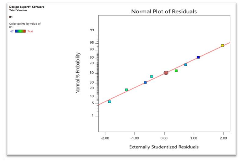
                     Figure 10: Normal plot of residual

Figure 10 seems there are no S shape curve generated and all the data close to a straight line. It means the data are normally distributed.

            Figure 11: Residual vs Predicted data of the model-2
There is no megaphone pattern appear in the residual vs predicted plot. It means their spread (variance) for different predicted values are constant. Therefore, the model is appropriate and no transformation needed.

Contour Plot for temperature-substrate concentration model As the model is found significant, the interference between temperature and substrate concentration can be drawn from the following 3D contour plot which is generated by the software.

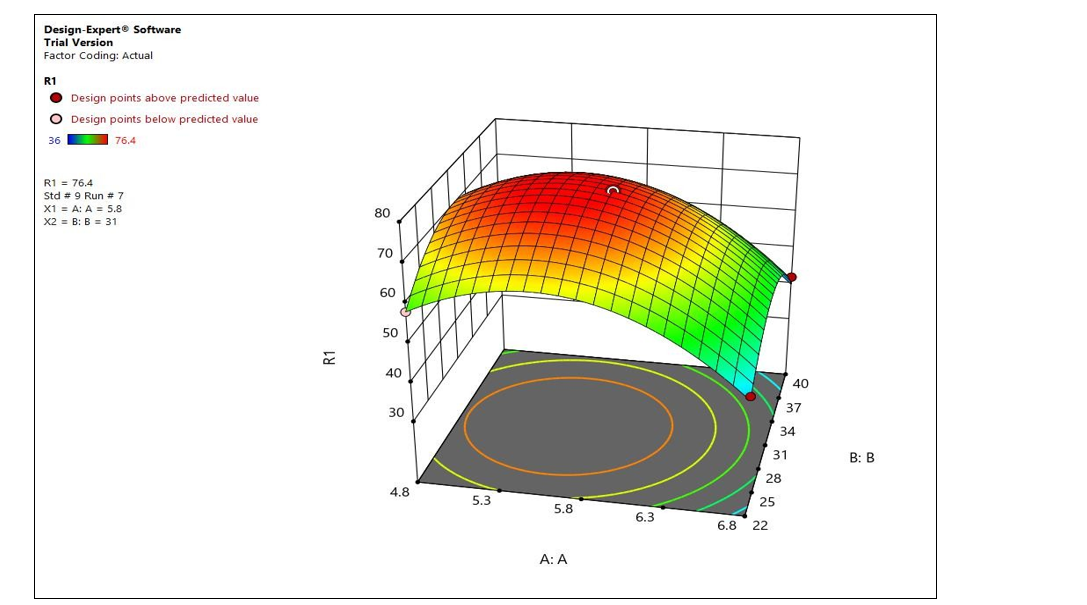
Figure 12: contour plot showing the effect of temperature and substrate concentration on ethanol production.

The figure shows the curvature which implies the importance of quadric equation. So the equation involves A2 and B2 are rightly selected. If the relationship will be linear, only a flat surface would appear. This curvature can be rotated to get different amount of ethanol production while changing the pH and temperature. Also the effect of temperature is more significant than substrate concentration due to lower P value. The software will also generate the numeric solution of the optimization. Numeric solution of optimization for temperature-substrate concentration model at figure 13.

Figure 13: Optimization of temperature and substrate concentration for maximizing the ethanol concentration

Optimization by Varying Substrate Concentration and pH

Table 11: The combined effect of pH and substrate concentration on ethanol production [21]                

 Final Equation in Terms of Coded Factors:

Y = +74.60 − 7.43A− 2027B + 0.53AB −14.47A² − 6.07B_²

Where, A=pH, B=Substrate concentration, Y=Ethanol concentration.

 Analysis of variance of model-3 (pH and substrate concentration)

                                           Table 12: Analysis of variance (ANOVA) of quadric model 3 [21]   

The ANOVA table underscores a significant model, highlighted by an F-value of 69.71 and a p-value of 0.0216, indicating strong statistical support for the model's predictive capability. P values are less than 0.05 and F value are larger than critical values. The quadratic effects of pH (F-value: 245.13, p-value: 0.0007) demonstrate a more pronounced significance than substrate concentration, pointing to pH as a critical factor in influencing the response variable. With an Adequate Precision ratio of 23.849, the model exhibits a robust signal-to-noise ratio, suggesting reliable

predictive performance. The model further shows the importance of quadric affect of pH is more significant than substrate concentration. The model's validity is further affirmed by the significance of both pH and substrate concentration, though with varying degrees of impact, necessitating further analysis through statistical distribution and transformation to ensure accuracy. Statistical distribution and transformation analysis for pH and substrate concentration model is shown at figure 14.

Figure 14: Normal plot of residual

Here it seems there are no S shape curve generated and all the data close to a straight line. It means the data are normally distributed.

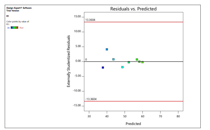
Figure 15: Residual vs Predicted data of the model-3

There is no megaphone pattern appear in the residual vs predicted plot. It means their spread for different predicted values are constant. Therefore, the model is appropriate and no transformation needed.

 Contour Plot for pH and Substrate Concentration Model As the model

is found significant, the interference between temperature and substrate concentration can be drawn from the following 3D contour plot which is generated by the software.

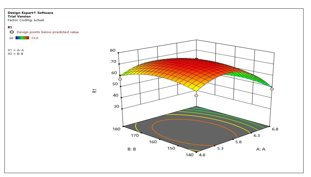
Figure 16: contour plot showing the effect of pH and temperature on ethanol production.

Like the previous couple of models, this pH-substrate model has also the curvature into its contour plot. Therefore, the relation between the two factors is not only linear, but also quadratic. The P value of temperature is lower than that of the temperature. Therefore, the effect of temperature is more pronounced.

Numeric optimization of ethanol by varying pH and substrate concentration are plotted below.

Numeric Solution of Optimization for pH and Substrate Concentration Model

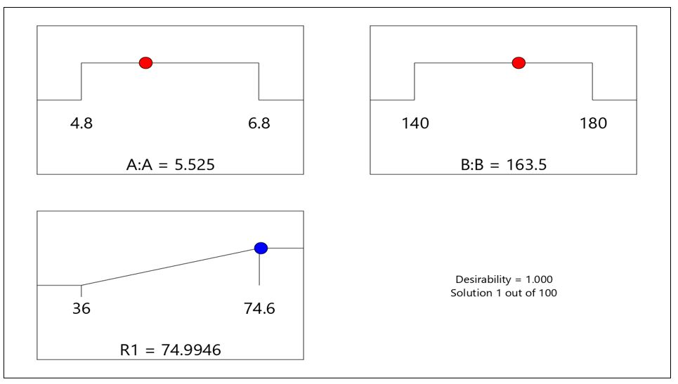
Figure 17: Optimization of pH and substrate concentration for maximizing the ethanol concentration

The optimization analysis for ethanol production, focusing on the interaction between pH, temperature, and substrate concentration, states significant insights into process enhancement through a quadratic model and ANOVA. However, this model's limitations include assumptions and simplifications that might not capture complex biological and chemical dynamics fully, with potential oversimplification of higher-order interactions.

The experimental design's finite parameter ranges and intervals can be further modified for optimal conditions, affecting the model's comprehensiveness. While statistical significance indicates model reliability, translating these findings into practical, large-scale applications necessitates evaluating the operational and cost implications, considering statistical significance may need to be adjusted for substantial industrial benefits. External

variability from biological systems, feedstock quality, and environmental factors are not considered in the current model, which can influence ethanol yield and quality. Additionally, the model's applicability can be scaled up by addressing challenges like heat and mass transfer effects or process control intricacies inherent in larger-scale operations. These constraints can be further investigated to refine the model, explore a wider array of parameters, and incorporate real-world variability and scaleup considerations for more accurate, applicable optimization strategies in corn to ethanol production.

Conclusion

This study approaches an optimization of ethanol production from corn, utilizing an unique approach that integrates PROII simulation results with statistical analysis via Response Surface Methodology (RSM). The PRO-II simulation delineates an optimized ethanol yield, achieving 92 wt% purity from a starting concentration of 90 g/L starch, translating to a increased production efficacy. Coupled with RSM's statistical validation the comprehensive analysis demonstrates a statistically significant impact of pH, temperature, and substrate concentration on ethanol production, highlighted by F-values (310.89 for pH and temperature; 89.23 for temperature and substrate; 69.71 for pH and substrate) and corresponding p-values (0.0036, 0.0021, and 0.0216, respectively) that affirm model validity. The first model underscores the significance of pH over temperature, while the second model emphasizes temperature over substrate concentration, and the third model highlights pH as more crucial than substrate concentration. Notably, the quadratic relationships identified signify the nuanced interactions between these variables, underscoring the efficacy of the Response Surface Methodology (RSM) in optimizing bioethanol production parameters. Our simulation results, revealing optimal conditions (pH 5.24-5.52, temperature 30-31°C, substrate concentration 158-163 g/L) for maximizing ethanol yield, further validate the models' predictive accuracy. This study's findings, supported by Adequate Precision ratios exceeding the threshold of 4, indicate a robust model capability in navigating the design space for ethanol production. Model comparisons reveal varying degrees of importance among pH, temperature, and substrate concentration. As the number of variables increases, future investigations may benefit from full factorial or fractional factorial designs to assess statistical models and conduct optimizations. Throughout this study, ethanol emerges as a promising energy source with lower carbon emissions, particularly relevant for enhancing domestic energy independence. While corn-to-ethanol processes are expanding in the US, economic success hinges on factors such as corn and ethanol prices. This well-established process, although requiring refinement, presents opportunities for enhancing enzyme efficiency, converting more material to ethanol, developing dedicated yeast for fermentation, and optimizing energy and water use. Despite drawbacks, including natural gas or coal consumption, CO2 emissions during fermentation, and water usage, ethanol remains a viable and relatively safe option for alternative energy, making a substantial contribution to minimizing reliance on conventional fuels for transportation and energy

References

- DOE Energy Information Administration. http://www.eia. doe.gov/fueloverview.html
- Renewable Fuels Association "Home Grown Energy," Ethanol Industry Outlook - 1999 and Beyond.
- Raphael Katzen Associates, (1979) Grain Motor Fuel Alcohol Technical and Economic Assessment.
- Ethanol. NIST: (2011). http://webbook.nist.gov/cgi/cbook. cgi?Units=SI&Name= ETHANOL
- Ethanol. Kirk-Othmer Encyclopedia of Chemical Technology (2004), Wiley & Sons.
- Ethanol. Coskata, Inc: (2011). http://www.coskata.com/ ethanol/index.asp?source= EE3777CF-954D-4610-9FDA-CAA6F5166155
- Alcohol Fuels. Kirk-Othmer Encyclopedia of Chemical Technology, (2000). Wiley & Sons.
- Ethanol Fuel Basics. Alternative Fuels Data Center. http:// www.afdc.energy.gov/fuels/ethanol_fuel_basics.html
- Air Quality Impacts of Increased Use of Ethanol Under the United States’ Energy Independence and Security Act. EPA Office of Transportation and Air Quality, 2010
- Ethanol Production. Alternative Fuels Data Center. http:// www.afdc.energy.gov/fuels/ethanol_production.html
- Alternative Fuels Data Center. http://www.afdc.energy.gov/ data/10328
- Mueller, S., Cuttica, J. J. (2006). Research investigation for the potential use of Illinois coal in dry mill ethanol plants Illinois.
- Macedo, I. C., Nogueira, L. A. H. (2005). Evaluation of ethanol production expansion in Brazil, section 2. Brasilia, Brazil: Nu´ cleo de AssuntosEstrate´gicos da Presideˆncia da Repu´ blica.
- Maranhao, L. E. C. (1982). Individual bagasse drier. US Patent 4326470.
- Clark, B. Ethanol. ICIS Chemical Business, (2013).
- Alternative Fuels Data Center. http://www.afdc.energy.gov/ data/10342
- Design of an Ethanol Fermentation Plant http:// ksmleadership.com/wp-content/uploads/2015/06/ Schrilla_J_Spring_2015.pdf
- Fermentation. Kirk-Othmer Encyclopedia of Chemical Technology (2004) Wiley & Sons.
- Benjamin, L., Xuesong, Li. Bioethanol from Starch Process Simulation Tutorial on PRO II/8.2
- Walia, N. K., Sekhon, K. K., Chaudhary, D. P., Cameotra,S. S., Srivastava, P., & Kumar, A. (2014). Optimization of fermentation parameters for bioconversion of corn to ethanol using response surface methodology. J Pet Environ Biotechnol, 5(3), 178.
- Kunamneni, A., & Singh, S. (2005). Response surface optimization of enzymatic hydrolysis of maize starch for higher glucose production. Biochemical Engineering Journal, 27(2), 179-190.
- Chen, Q. H., He, G. Q., & Ali, M. A. (2002). Optimization of medium composition for the production of elastase by Bacillus sp. EL31410 with response surface methodology. Enzyme and microbial Technology, 30(5), 667-672.
- Mathewson, S. W. (1980). The manual for the home andfarm production of alcohol fuel. Danvers, MA: Ten Speed Press
- Tahir, A., & Aftab, M. (2010). Effect of cultural conditions on ethanol production by locally isolated Saccharomyces cerevisiae BIO-07. Journal of Applied Pharmacy, 2, 72-78.
- https://www.grainprocessing.com/alcohol/alcohol-grades. html
- http://iopscience.iop.org/ article/10.1088/1748-9326/2/2/024001/meta
- https://afdc.energy.gov/data/10342
- http://www.eia.gov/forecasts/aeo/er/tables_ref.cfm
- E85Prices. http://www.e85prices.com
- https://blog.processsystemsdesign.com/2017/07/the-ethanol-production-process.html
- https://www.e-education.psu.edu/egee439/node/673
- https://www.agmrc.org/renewable-energy/renewable-energy-climate-change-report/renewable-energy-climate-change-report/november-2017-report/chinas-new-ethanol-use-mandate-will-create-opportunities-for-us-exports
- http://www.ers.usda.gov/media/866543/cornusetable.html
- BiaÅ?as, W., Czerniak, A., & Szymanowska-PowaÅ?owska, D. (2014). Kinetic modeling of simultaneous saccharification and fermentation of corn starch for ethanol production. Acta Biochimica Polonica, 61(1), 153-162.
- Renewable Fuels Association. (2023). New Study: Ethanol Industry’s Impact on the U.S. Economy Strengthened in 2022.
- S&P Global. (2022). Commodities 2023: Ethanol plants in US to face hard choices.
- Irwin, S. (2024). Trends in the Operational Efficiency of the US Ethanol Industry: 2023 Update. farmdoc daily, 14(28).
- Occupational Safety and Health Administration, Flammable liquids. https://www.osha.gov/laws-regs/regulations/ standardnumber/1910/1910.106
- National Fire Protection Association. NFPA 30: Flammable and combustible liquids code.
- Legal Information Institute. 40 CFR § 280.32 - Compatibility.
- ePURE. "Beverage & Industrial Use." (2024).
- U.S. Energy Information Administration (EIA). "Ethanol Explained." 2024.
- Douglas, L. (2022). "U.S. corn-based ethanol worse for the climate than gasoline, study finds."
- "The Case Against More Ethanol: It’s Simply Bad for Environment." Yale Environment 360.
- "Biofuels and Water Use: Background, Issues, and Trends." National Renewable Energy Laboratory (NREL).
- Lin, T. S., Kheshgi, H. S., Song, Y., Vörösmarty, C. J., & Jain, A. K. (2023). Which crop has the highest bioethanol yield in the United States?. Frontiers in Energy Research, 11, 1070186.
- Irwin, S. (2024). Another Strong Year for Ethanol Production Profits in 2023. farmdoc daily, 14(29).
- Sree, N. K., Sridhar, M., Suresh, K., & Rao, L. V. (1999). High alcohol production by solid substrate fermentation from starchy substrates using thermotolerant Saccharomyces cerevisiae. Bioprocess engineering, 20, 561-563.
- Balat, M., Balat, H., & Öz, C. (2008). Progress in bioethanol processing. Progress in energy and combustion science, 34(5), 551-573.
- Aden, A., Ruth, M., & Iechura, J. (2002). Lignocellulosic Biomass to Ethanol Process Design and Economics Utilising Co-current Dilute Acid Prehydrolysis and Enzymatic Hydrolysis for Corn Stover. National Renewable Energy Laboratory (NREL) Report TP510-32438
- U.S. Department of Energy. Ethanol Fuel Basics.