
Journal of Electrical Electronics Engineering(JEEE)
ISSN: 2834-4928 | DOI: 10.33140/JEEE
Impact Factor: 1.2


Research Article - (2023) Volume 2, Issue 4
Centrality Measures to locate the COI of the Mexican Electricity Grid
Research Article J Electrical Electron Eng, 2023 Volume 2 | Issue 4 | 565-570; DOI: 10.33140/JEEE.02.04.22
Juan M. Ramirez*
*Electrical Engineering Department, CINVESTAV – GDL, Zapopan, Jal. MEXICO, 45019
*Corresponding Author : Juan M. Ramirez, Electrical Engineering Department, CINVESTAV – GDL, Zapopan, Jal. MEXICO, 45019.
Submitted: 2023, November 13; Accepted: 2023, December 04; Published: 2023, December 26
Citation: Ramirez, J. M. (2023).Centrality Measures to locate the COI of the Mexican Electricity Grid. J Electrical Electron Eng, 2(4), 565-570.
Keywords: Center of Inertia, Centrality Measure, Frequency Control, Power System Control
Abstract
Centrality measures based on network topology are valuable for decision-making in complex systems. These measures allow the identification of the most essential elements of the network, i.e. those that have the most significant impact on the overall operation of the system. In the case of electricity grids, centrality measurements can be used to identify the most crucial power plants, the most critical transmission lines, or the most vulnerable connection points. This information can be used to improve network planning and control to ensure a reliable and secure electricity supply. In this paper, centrality measures are used to identify those nodes in the Mexican electricity network that are topologically the most relevant. These are used to locate frequency meters that act as critical points for frequency control. Results are presented for an equivalent network of 190 busbars divided into geographical control regions.
Keywords:
Center of Inertia, Centrality Measure, Frequency Control, Power System Control
1. Introduction
The mathematical study of complex networks that real-world model problems has had significant advances: on the one hand, the spectral theory of graphs, which uncovers valuable information on the topological structure of networks encoded in the eigenvalues and eigenvectors of matrices associated with the networks, and on the other hand, the study of the temporal evolution of networks that motivated the introduction of the concept of scale-free networks, which have been identified as those that are formed in the interaction of human societies.
This paper considers a reduced equivalent of the national electricity grid consisting of 190 busbars and 46 generating units. The graph theory and matrix analysis techniques allow us to define centrality measures that determine the vertices' relative importance from the graph topology. Such information is strategic in problem-solving. Our attention will concentrate on three centrality measures: closeness, PageRank, and spectral centrality.
We also consider graphs representing the national power grid. Graph theory techniques allow us to define centrality measures that determine the relative importance of each vertex in the graph. Two centrality measures will focus our attention: closeness, which determines the rank of the proximity of a node to the others in the network; PageRank; and spectral, determined according to the coordinates of a positive eigenvector called Perron's, associated with the maximum value of the matrix considered (usually adjacency or weighted adjacency).
The concept of centrality measures was first introduced by A. Bavelas in the 1950s in the context of the social sciences [1]. It has been one of the most studied terms in network analysis since the late 1970s. Some authors have used centrality measures concerning the flow of information in various networks, the flow of used goods, the movement of money, the spread of rumours, e-mails, attitudes, and infections, and the direction of packets.
Although centrality measurements have been used for many years for applications in electrical networks, they usually have been used with aspects related to voltage problems. Here, we will do it instead for frequency problems, which are vital in the Mexican grid operation nowadays.
Our network analyses point in one direction: to identify the power grid's main busbars from a topological point of view. With this, we consider installing measurements at such nodes vital, for example, for the study system's frequency.
2.Graph Metrics
This section shows the most commonly used metrics in graph analysis. These are of great help in understanding the behavior of the network.
● Degree: The degree of a vertex in a graph G = (V, E), denoted Ku, where u is a vertex u ∈ V; it is the number of proper edges incident on the vertex, plus twice the number of loops existing at the same vertex. The degree can also be calculated by counting the number of neighboring vertices of the vertex under analysis.
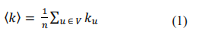
The calculation of the average degree gives a clearer idea of the degree of the network as a whole. It can be easily calculated with the following equation:
Another way to analyses a graph from the degree is to plot its degree distribution. This gives the probability that a selected vertex in the graph has a degree k. For a graph with n vertices, the degree distribution is given by the following equation.
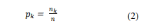
where nk is the number of vertices with k-degrees.
● Density: The density indicates the proportion of edges that a graph possesses. If the density is high in the graph G, then the number of edges in the graph G is close to the maximum possible number of edges, i.e. the number of edges in a complete graph. In the opposite case, a low density in the network G indicates that the network has very few existing connections. For a graph with n vertices and m edges, the equation to calculate the density is the following,

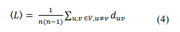
● Shortest Path: The Shortest Path Length of a graph refers to the shortest distance between a pair of vertices. If the network is weighted, the distance calculation is computed through the sum of the weights indicated by each edge selected as part of the shortest path. If the network is unweighted, the calculated distance is called the geodesic distance, where the weights of all edges are equal to one. The average shortest path distance is the average of all distances duv in G,
Dijkstra's algorithm is often used to obtain the shortest path between two vertices. Dijkstra's algorithm solves the problem of finding the shortest path between nodes in a weighted graph G = (V, E) in which all weights must be positive [2]. The algorithm starts from the selected node (source node) and performs a search in the network to achieve its goal: to find the shortest path between the selected node and the other nodes in the network. During its execution, it stores the shortest path found so far between each node and the source node; if it finds a shorter path, it updates it. When the algorithm finds the shortest path between the source node and another node, the node is marked as "visited" and added to the stored shortest path. This continues until all nodes in the network have been added to the path. This way, you have a path connecting the originating node to the other nodes via the shortest possible path.
● Diameter:TThe diameter of a graph G is the maximum shortest path between two vertices. With this metric, we can observe the distance between the farthest vertices in the graph.
● Clustering Coefficient:The clustering coefficient measures how connected the neighbours of a vertex are. When its value is high, there is a strong connection between the neighbours of a vertex, and when its value is low, there is a low connection between neighbors. For a vertex u with degree ku, the clustering coefficient is defined as follows,
● Clustering Coefficient:The diameter of a graph G is the maximum shortest path between two vertices. With this metric, we can observe the distance between the farthest vertices in the graph.
Where Eu is the number of edges in the subgraph created by the set of neighbours of vertex u.
The above equation shows the local clustering coefficient, i.e., each vertex's clustering coefficient; however, obtaining its global value is more interesting, which helps to understand the behaviour of the network. This can be easily calculated by obtaining the average through the local clustering coefficient of the network,
An incidence matrix is a binary matrix (i.e. its elements can only be ones or zeros) used to represent binary relationships. In particular, it represents graphs and mathematical structures that model relationships between objects. An incidence matrix of a graph has as many rows as there are vertices and as many columns as there are edges in the graph. The matrix element in row i and column j is one if vertex i is incident to edge j and zero otherwise.
Complex networks In the open research, the terms network and graph are used interchangeably. As mentioned above, a complex network is commonly a graph representing a system with abundant complex entities and interactions. The study of complex networks helps to understand various real systems. For example, we can understand the behavior of neurons connected by synapses or even the Internet, which comprises routers, cables and optical fibers. These systems are called complex systems since predicting their collective behavior through their components is impossible. However, by analyzing the properties of the network, it is possible to predict and even control them [3]. Complex networks are the graphs that represent these complex systems. A complex network is a graph with abundant nodes with specific properties and behavior. Thus, in this work, the applications are in the context of electricity grids, which can be considered complex grids.
3. Used Centrality Measures
A centrality function (fG) assigns a positive real value to each node of a network G such that if g: G→G' is an isomorphism, then fG(x)=fG'(g(x)) for all x nodes of G. Thus, the centrality function is a structural attribute of the nodes in a network; in other words, it is a value assigned to the node due to its structural position in the network.
In this paper, the following centrality measures are utilized. These were chosen because they are widely used and well established.
● Weighted Degree: This is the first and most straightforward definition of centrality. It is defined as the number of (weighted) links a node has with other nodes. It is usually represented as k. The degree is often interpreted as the number of connections a network element has.
where the line-node (m lines, n nodes) incidence matrix A, with size m × n, is used to calculate the Laplacian matrix L of the network, with size n×n, as L=ATA.
● PageRank: The function of this algorithm is to measure the importance and quality of a web page in a range from 0 to 10; it follows a series of measurable criteria.
Google's PageRank is inspired by the Science Citation Index (SCI), the world's best-known citation index. The SCI measures the importance of different scientific publications, determining their relevance and influence based on the references they have received from other publications.
The PageRank value of a web page is determined by the links from other pages and their quality. That is the quality of the pointing domain, its age, and the importance given to each connection. This does not mean that a page with many links has a PageRank of 10 since it will receive a low score if the links are of low quality. In practice, it means that a web page that receives links from pages with a good PageRank - those pages that Google considers high quality and authoritative-will have a high PageRank. Still, if the majority are low-quality links, it will have a low PageRank.
(i) Eigenvector centrality: If A is a symmetric matrix, i.e., aij = aij, for all entries 1 ≤ i, j ≤ n, then there are n real solutions of its characteristic equation det (λI-A)=0. In case the matrix A is non-negative, i.e., aij ≥ 0 for all entries i, j, then there are eigenvalues λ ≥ 0:
is called the spectral radius of A.
In 1907, the German mathematician Oskar Perron proved the following theorem: Let A= (aij) be a nonnegative matrix and let r be its spectral radius, then:
● λ is an eigenvalue of A;
● there exists an eigenvector u of A such that Au = λu and all entries of u are non-negative;
● if A is the adjacency matrix of a connected graph, then they hold:
(a) λ is a simple root of the characteristic polynomial of A and
(b) the vector u has all its entries greater than zero.
If G is a connected graph and A is its adjacency matrix, the values u(x) for x node of G determine the spectral centrality function. Therefore, we interpret u(x) as a measure of the complexity of the network G at node x.
4.Case Study
In this section, we assume linearised models for representing the dynamics of the Mexican Interconnected System (MIS), whose primary purpose is to quantify the frequency deviations in the different regions that comprise the system. Furthermore, through centrality measurements, it is desired to identify the central nodes of the network from a topological point of view to recommend the measure of such nodes as critical for frequency control.
In the present analysis, studies are carried out on the MIS dynamic model, which represents the transmission voltage levels, Fig. 1. A typical operating point for the system is used. One hundred fifty-eight generators and 2022 high-voltage nodes comprise the network and are spread over the MIS's seven regions. The working condition hinges on the 2018 base case [4]. Due to a lack of technical information, some plants were not considered in the study because they are privately owned.
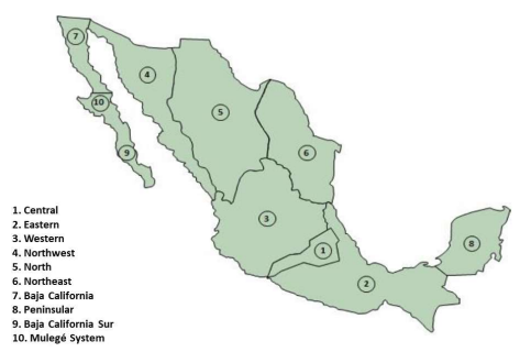
Figure 1:Geographical divisions for the control of the Mexican electricity grid.
Spreading from Central America to the United States border, the MIS encompasses seven control areas working synchronously. These are here identified as Northwest (NW), North (N), and Northeast (NE). The systems selected were West (W), Central (C), Southeast (SE), and Peninsular (P). The system is of the longitudinal type, with the operational implications that this implies. Consequently, dynamic safety is usually an issue [5].
The center of inertia is an essential point in studying the mechanics of solids. It is defined as the point at which the mass of a body is considered to be concentrated. This is of utmost importance in studying the dynamics of solids since it is the point around which all motions occur. The centre of inertia is also used to calculate the body's moment of inertia, which measures its resistance to change its angular velocity. This is important for the design of machinery, where manufacturers must take the moment of inertia into account to ensure that the machine is strong enough to resist the force of the movements. In our application, by analogy with the concept of the centre of inertia of a solid body, the electrical system's centre of inertia (COI) is considered here to represent a binding site through which the frequency variation travels.
4.1 Followed Procedure and Results
The first step in calculating the different centrality measures is to create a graph for the network topology under study. A graph is an abstract data structure that uses nodes to represent objects and lines to describe connections between them. Graphs are also networks, as the nodes are connected to form a network of information. Networks are useful for modelling relationships between objects and analysing network-related problems.
In this case, the network has 190 busbars and 264 transmission lines, representing an equivalent of Mexico's high-voltage network. A weight is associated with each transmission line. Two different weights were chosen: (i) the absolute value of the series impedance of the line and (ii) the absolute value of the flow through it. With this information, the undirected weighted graph, G, is constructed for the network under study. In an undirected graph, an edge has no direction associated with it. Thus, if there is a link between vertices A and B, there is also a connection between vertices B and A.
Once the corresponding network is available, the centrality measures described in section 2 are calculated. Table 1 shows the ranking of the selected nodes for each measurement. Notably, the results coincide for the impedance-weighted and flow-weighted networks for the first eight nodes of the ranking.
| Degree | PageRank | Eigenvector |
|---|---|---|
| 96 | 96 | 96 |
| 78 | 53 | 68 |
| 64 | 143 | 131 |
| 53 | 64 | 88 |
| 89 | 78 | 89 |
| 185 | 158 | 78 |
| 158 | 128 | 100 |
| 143 | 110 | 90 |
Table 1: The first eight nodes ranked by the centrality measures used.
Table 1 shows a set of matching nodes for the different centrality measures (53, 78, 96, 143). Node 96, the first-ranked node in all three cases, is particularly noteworthy. This node corresponds to the central control area, close to the metropolitan area of Mexico City.
Demand increase simulations are carried out at some nodes of the different control areas to verify the reliability of the nodes selected by the centrality measures. In this case, there is a particular interest in observing frequency at other nodes of such area, at the COI, and node 96 selected first, according to Table 1.
The simulations were carried out with fourth-order models for the synchronous machines, each equipped with a simple exciter and speed governor (eight state variables for each generator). First, the frequency at the load buses is estimated with a Phase-Lock-Loop (PLL) model, representing two state variables each. The event that gives rise to the frequency modification is the increase in demand at load nodes, and the frequency signal is observed at different nodes of the network, including the COI, calculated according to the following expression,
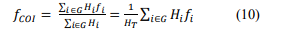
where G stands for the set of synchronous generators, fi is the frequency associated with each element of G, and Hi represents the corresponding inertia; HT is the total inertia.
In this case, the root means squared error RMSE is used to compare pairs of curves. If they were identical, the RMSE would be zero. The higher the RMSE value, the more differences between the compared curves within the observation interval. The definition of the RMSE indicates that,
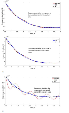
Figure 2:Frequency deviation behaviour after an increase in demand in (a) eastern area, (b) central area, (c) western area.
Figure 2 illustrates the frequency behaviour, measured from different buses, after an increase in demand (i) in the eastern control area (5% increase on buses 83 and 84) and (ii) in the central control area (5% increase on buses 109 and 110). Initially, the system is in a steady state. Then, three frequency curves are presented: (a) the arithmetic average of the frequencies measured at all area's load buses; (b) the COI; (c) the measurement at bus 96.
where Oi are the observations, Si predicted values of a variable, and n is the number of observations available for analysis.
In this application, since the values of the frequency deviations are minimal (in Hz), Fig. 2, it was considered relevant to express the RMSE values of Table 2 in pu, where 1 means the smallest RMSE value within the analysed case, concerning the COI.
| Case 1 (fig 2a) | Case 2 (fig 2b) | Case 3 (fig 2c) | |
|---|---|---|---|
| Average-COI | 1 | 1 | 4.39 |
| Bus 96-COI | 2.60 | 1.01 | 1 |
Table 2: RMSE values referenced to the COI.
Simulations were carried out for the other control areas; they are not presented for brevity. As can be seen from the frequency behaviour, the COI curve is smooth (no oscillations), which is not strictly valid for an existing system. The curve corresponding to bus 96 resembles the COI curve, indicating that this node is physically very close to the COI. It cannot be precisely the COI because it is very likely that more nodes would have to be included in the network to get closer to the actual centre. Nevertheless, it is considered that the results found with the centrality measures used provide an excellent location of the valid COI.
5. Conclusion
Measurements are an essential tool for network diagnostics and monitoring. They help verify the operating quality, detect problems, identify trends, and predict results. Frequency measurements are crucial because they help provide valuable information on their behavior. This information is used to make control decisions, improve operations, provide quality service to users, and optimize efficiency.
Taking measurements in the right place is essential to obtain accurate results. This involves placing measurement equipment in the right place at the right time to collect accurate information. This has been the object of this paper: to identify, through centrality measures, those topologically appropriate busbars to locate frequency measurements to reduce the installation of PMUs without losing valuable information.
For the case of the Mexican network, the results are considered valid in identifying the location of the COI.
Acknowledgements
Juan M. Ramirez acknowledges support from SENER-CONACyT Project FSE-2013-05246949.
References
- Bavelas, A. (1950). Communication patterns in task‐oriented groups. The journal of the acoustical society of America, 22(6), 725-730.
- Cormen, T. H., Leiserson, C. E., Rivest, R. L., & Stein, C. (2022). Introduction to algorithms (Fourth).
- Mata, A. S. D. (2020). Complex networks: a mini-review. Brazilian Journal of Physics, 50, 658-672.
- Freeman, L. C. (1979). Centrality in social networks: Conceptual clarification. Social network: critical concepts in sociology. Londres: Routledge, 1, 238-263.
- Energy Secretariat MEXICO. (2019). Program for developing the national electricity system PRODESEN 2019-2033 (in Spanish).
Copyright:
Copyright: ©2023 Juan M. Ramirez. This is an open-access article distributed under the terms of the Creative Commons Attribution License, which permits unrestricted use, distribution, and reproduction in any medium, provided the original author and source are credited.