Artificial Neural Networks in The Perception of Genetic Differentiation Caused by Migration

Introduction

The maintenance of genetic diversity is a essential factor for the conservation of population viability, and this can be measured by the genetic differences among individuals [1]. Genetic variability is based on the differentiation of allelic and genotypic frequencies among individuals of a particular population [2]. In this way, genetic diversity plays a key role in contributing to biodiversity by ensuring the evolution and adaptation of species to their environments.

Populations lacking genetic variability are more predisposed to extinction. This genetic variability arises due to various evolutionary mechanisms acting on populations such as migration. According to Salman, migration can be defined as: "a transferf requency (q₂) to another reproducing population with a different gene frequency (q₁₎" [3]. Therefore, migrants bring new alleles and consequently increase genetic diversity within the population, reducing the differences between populations. One way to map the changes generated by evolutionary factors is through multivariate techniques capable of organizing genetic diversity and highlighting the effects caused by them, such as Self-Organizing Maps (SOM) [1]. 

Self-Organizing Maps (SOM) is a type of artificial neural network capable of organizing input information into a two-dimensional map through an unsupervised learning process that preserves neighborhood relationships using Euclidean distance [4]. Self- Organizing Maps (SOM) neural networks have the ability to organize subpopulations based on the level of similarity between them in a topological manner on a two-dimensional map. This facilitates visualization and observation across generations regarding the effects of genetic diversity for easier analysis [5]. In light of this, understanding the characteristics and applicability of SOM techniques is crucial, as it is a tool that provides additional information beyond what is generated by traditional approaches in the study of genetic diversity [1]. Hedrick's statistics take into account only genotypic frequencies, while Nei's statistics are based on gene or allelic heterozygosity and allow for the calculation of diversity both within and among populations, subpopulations, and various hierarchical levels of classification [6]. Although conventional biostatistics techniques group data, they do not provide enough information to determine the relationship between these groups. On the other hand, SOM does not form groups like conventional techniques, but it can organize less divergent populations within the same neuron and group such neurons closer on a map. For this reason, it's not possible to directly compare SOM with traditional clustering methods; instead, traditional methods serve as a reference point to assess the coherence of SOM [7].

Given on above, the objective of this study was to investigate the effects of migration over generations, analyzing them using Conventional Biostatistics Techniques - Nei's Statistics, Hedrick's Statistics, and Tocher's Clustering - and subsequently, to assess whether self-organizing maps are capable of mapping the effects caused by migration.

Methodology

In the Genetic and Experimental Statistics Software Portal Genes [8], base populations, donor populations (D), and receptor populations (R) were generated in Hardy-Weinberg equilibrium, each with 1000 individuals, 100 diallelic loci with codominant markers, and variable allelic frequencies (0 ≤ p ≤ 1). Hardy- Weinberg Equilibrium (HWE) represents idealized populations that are stable, with constant allelic and genotypic frequencies across generations. Using populations in HWE makes it easier to observe and understand any changes generated by migration during simulations. Starting from the base population in Hardy- Weinberg equilibrium, subpopulations were simulated under the influence of migration. Migrants (m = 50; m = 100; m = 300) left the donor population for the receptor population for 10, 15, and 20 generations, thus forming subpopulations (P1, P2, P3,...). These subpopulations were then analyzed using the Nei, Hedrick, and Tocher clustering techniques. Self-Organizing Maps (SOM) were created using Matlab 2016a software integrated with Portal Genes (Cruz 2016) and edited in MSOffice. The basic population descriptors (q, D, and H, representing the allelic frequencies of allele A2, the homozygous genotype for allele A1, and the heterozygotes) were used as input information. To confirm the findings that Self-Organizing Maps are more sensitive in detecting genetic variability and providing additional information to organize populations on maps, replication of simulations and analyses was conducted.

Os SOM apresentados nas figuras dos resultado e discussão forão construídos a partir das imagens created using Matlab 2016a software integrated with Portal Genes and edited in MSOffice [9].

Result and Discussion

In the study performed by Oliveira, Santos and Cruz, Self- Organizing Maps (SOM) were able to organize populations according to the biological principles of the simulated effects [6]. This was observed for populations subjected to processes that reduce variability, such as genetic drift, inbreeding, and selection, as well as for processes that increase variability, such as migration. In the simulation conducted under the effect of migration, the authors found that SOM was efficient in organizing populations subjected to migration. However, it's worth noting that these authors tested it only for the migration of 100 migrants over four generations. This suggests that SOM has the potential to effectively capture and represent the genetic changes resulting from migration, but further investigation may be needed to explore its performance under various migration scenarios and conditions.

Based on the methodologies of Oliveira, Santos and Cruz, we tested various numbers of migrants over different numbers of generations [6]. The number of migrants (m) ranged from 50 to 300 individuals, and the effect was simulated for g generations, with g ranging from 10 to 20 generations. The results obtained for each tested combination of m and g are described below.

For 50 migrants (m = 50) over 10 generations (g = 10), Nei's GST statistic and Hedrick's Genotypic Measure clustered by Tocher were unable to detect genetic variability between generations. They formed one group that included the receptor population and all generations of migration, and another group with only the donor population (Table 1a, 1b). Therefore, it was not possible to observe what was happening as more migrants arrived over the generations using these traditional statistics. On the other hand, the Kohonen map, also known as the Self-Organizing Map (SOM), was able to highlight more clearly how each generation behaved with m = 50. It was also possible to observe that there was a change between generations with the arrival of migrants because the subpopulations were allocated to different neurons (Figure 1A), although the distance between these neurons was small, as indicated by the light-yellow color between neurons (Figure 1B). This occurred due to migrants number (50) has generated minimal changes.

Table 1: a. Tocher optimization clustering for Nei's GST statistic under the effect of migration, with 50 migrants for 10 generations. b. Tocher optimization clustering for Hedrick's Genotypic Measure under the effect of migration, with 50 migrants for 10 generations

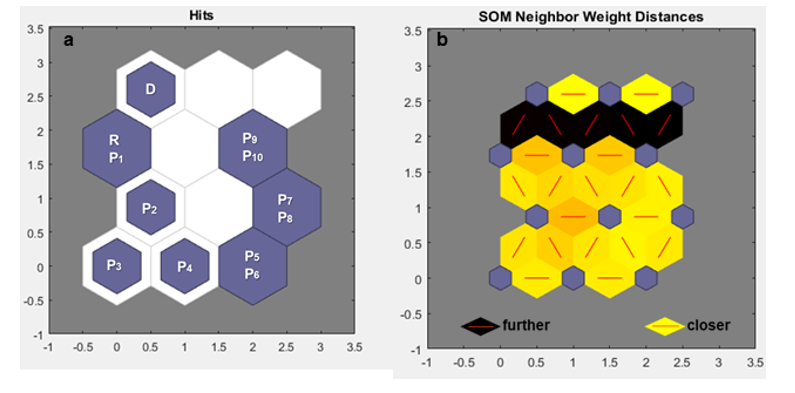
Figure 1: a. Mapping performed by the Self-Organizing Map (SOM) under the effect of migration, with the value of m = 50 for 10 generations, in a 4X3 neuron matrix (row X column). b. Distance mapping between neurons, based on coloration by SOM under the effect of migration, with the value of m = 50 for 10 generations, in a 4X3 neuron matrix (row X column). Donor base population (D); receptor base population (R); subpopulations (P1, P2, P3,...)

For the populations generated with migration involving 50 individuals (m = 50) over 15 generations (g = 15), Nei's GST statistic, Hedrick's Genotypic Measure clustered by Tocher, and the self-organizing maps exhibited the same pattern as for m = 50 for 10 generations, as observed earlier. The conventional methods were not effective in detecting genetic variability between generations, resulting in one group containing the receptor base population and the other subpopulations, and another group with only the donor base population (Table 2a, 2b). With self-organizing maps, it is possible to observe where each subpopulation is clustered and their respective neurons (Figure 2a), as well as the distance between these neurons (Figure 2b). Despite an increase in the number of generations, the number of migrants is still very low, and therefore, significant changes are not observed.

Table 2: a. Tocher optimization clustering for Nei's GST statistic under the effect of migration, with 50 migrants for 15 generations. b. Tocher optimization clustering for Hedrick's Genotypic Measure under the effect of migration, with 50 migrants for 15 generations

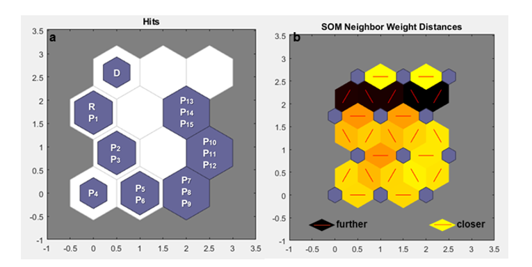
Figure 2: a. Mapping performed by the Self-Organizing Map (SOM) under the effect of migration, with the value of m = 50 for 15 generations, in a 4X3 neuron matrix (row X column). b. Distance mapping between neurons, based on coloration by SOM under the effect of migration, with the value of m = 50 for 15 generations, in a 4X3 neuron matrix (row X column). Donor base population (D); receptor base population (R); subpopulations (P1, P2, P3,...).

Maintaining 50 migrants (m=50) and increasing the effect to 20 generations (g = 20) made it possible to observe a difference compared to the previous results. Although 50 migrants did not have a significant impact on the population in the early generations, there was an impact in the later generations. Over 20 generations, Nei's GST statistic and Hedrick's Genotypic Measure clustered by Tocher were more efficient in highlighting genetic variability between generations, and both grouped the donor base population in group 3, the receptor base population in group 2, and the other subpopulation generations in group 1 (Table 3a, 3b). However, it is still not possible to clearly determine how close one subpopulation is to another. Nonetheless, the self-organizing maps were useful in making it more evident what occurred over the course of the 20 generations by highlighting, through colors, the distance between subpopulations (Figure 3b). However, even with the increase in generations, the receptor base population still occupies the same neuron as the subpopulation of the first generation, and they are still very distant from the donor base population (Figure 3a).

Table 3: a. Tocher optimization clustering for Nei's GST statistic under the effect of migration, with 50 migrants for 20 generations. b. Tocher optimization clustering for Hedrick's Genotypic Measure under the effect of migration, with 50 migrants for 20 generations

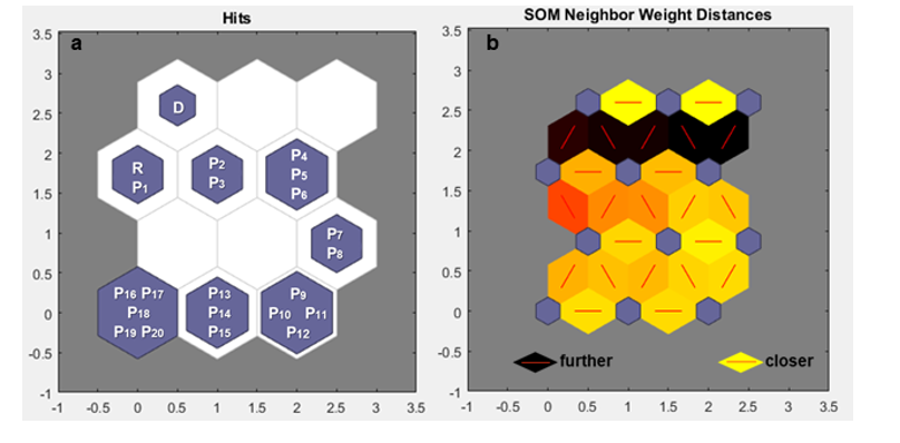
Figure 3: a. Mapping performed by the Self-Organizing Map (SOM) under the effect of migration, with the value of m = 50 for 20 generations, in a 4X3 neuron matrix (row X column). b. Distance mapping between neurons, based on coloration by SOM under the effect of migration, with the value of m = 50 for 20 generations, in a 4X3 neuron matrix (row X column). Donor base population (D); receptor base population (R); subpopulations (P1, P2, P3,...)

The Nei's GST statistic and Hedrick's Genotypic Measure grouped by Tocher, now for the values of 100 migrants (m = 100) over 10 generations, were able to more noticeably detect genetic variability between generations, separating the donor base population into one group, the receptor base population into another group, and the migration generations into another group (Table 2a, 2b). However, it was still not possible to observe what happened when more migrants arrived over the generations or to determine which subpopulations were closer or farther from each other using these conventional statistics. However, the Kohonen map was efficient in highlighting the effects caused by migration and how each generation behaved with m = 100. We were able to observe that the donor base population and the receptor base population were grouped in different and more distant neurons (isolated by the black color) (Figure 2a). In addition, it is evident that the maps generated for m = 100 for 10 generations are more colorful, indicating that with the arrival of more migrants, there was greater differentiation between the 10 generations.

Table 4: a. Tocher optimization clustering for Nei's GST statistic under the effect of migration, with 100 migrants for 10 generations. b. Tocher optimization clustering for Hedrick's Genotypic Measure under the effect of migration, with 100 migrants for 10 generations

Figure 4: a. Mapping performed by the Self-Organizing Map (SOM) under the effect of migration, with the value of m = 100 for 10 generations, in a 4X3 neuron matrix (row X column). b. Distance mapping between neurons, based on coloration by SOM under the effect of migration, with the value of m=100 for 10 generations, in a 4X3 neuron matrix (row X column). Donor base population (D); receptor base population (R); subpopulations (P1, P2, P3,...).

For the same number of migrants (m = 100) over 15 generations, Nei's GST statistic and Hedrick's Genotypic Measure clustered by Tocher grouped their subpopulations into four and three groups, respectively. Nei's GST statistic separated the donor base population into group 4, the receptor base population into group 3, subpopulations (1-5) into group 2, and subpopulations (6-15) into group 1 (Table 5a). On the other hand, Hedrick's Genotypic Measure separated the donor base population into group 3, the receptor base population into group 2, subpopulations (1-4) into group 2, and the remaining subpopulations (5-15) into group 1 (Table 5b).

Therefore, Nei's GST statistic was more effective in highlighting the effects caused by migration over generations compared to Hedrick's Genotypic Measure, but still not entirely sufficient. Once again, the Kohonen maps grouped the subpopulations differently from before: the donor base population is in the first neuron along with P15, and the receptor base population is in the third neuron along with P1, forming a curve (Figure. 5a). Additionally, both base populations are close to each other, and the other subpopulations are also very close to each other, as indicated by the shades of orange and light yellow in the maps (Figure 5b).

Table 5: a. Tocher optimization clustering for Nei's GST statistic under the effect of migration, with 100 migrants for 15 generations. b. Tocher optimization clustering for Hedrick's Genotypic Measure under the effect of migration, with 100 migrants for 15 generations

Figure 5: a. Mapping performed by the Self-Organizing Map (SOM) under the effect of migration, with the value of m = 100 for 15 generations, in a 4X3 neuron matrix (row X column). b. Distance mapping between neurons, based on coloration by SOM under the effect of migration, with the value of m = 100 for 15 generations, in a 4X3 neuron matrix (row X column). Donor base population (D); receptor base population (R); subpopulations (P1, P2, P3,...).

For the same number of migrants (m = 100) but over 20 generations, Nei's GST statistic and Hedrick's Genotypic Measure grouped by Tocher clustered their subpopulations into five and six groups, respectively. Nei's GST statistic separated the donor base population into group 5, the receptor base population and subpopulations (1 and 2) into group 4, subpopulations (6-10) into group 2, and subpopulations (11-20) into group 1 (Table 6a). On the other hand, Hedrick's Genotypic Measure separated the donor base population into group 6, the receptor base population into group 5, subpopulations (1 and 2) into group 4, subpopulations (3-5) into group 3, subpopulations (9-10) into group 2, and subpopulations (11-20) into group 1 (Table 6b). For m = 100 over 20 generations, Nei's GST statistic and Hedrick's Genotypic Measure were even more effective, separating the subpopulations into a greater number of groups. This time, Hedrick's Genotypic Measure was more effective in highlighting the effects of migration over generations compared to Nei's GST statistic, as it managed to separate them into more groups and distinguish the receptor base population from the other subpopulations. The Self- Organizing Maps grouped the donor base population in the tenth neuron and the receptor base population together with P1 in the seventh neuron. They also grouped the other subpopulations in the fourth, first, second, third, sixth, and ninth neurons, forming a curve that approaches the donor base population again (Fig. 6A). Additionally, it is evident that the donor base population and the receptor base population are very distant from each other, with the black color indicating their separation. The red color between the seventh and fourth neurons suggests they are closer but still distant, and the other neurons are closer to each other, indicated by the yellow color (Figure. 6b).

Table 6: a. Tocher optimization clustering for Nei's GST statistic under the effect of migration, with 100 migrants for 20 generations. b. Tocher optimization clustering for Hedrick's Genotypic Measure under the effect of migration, with 100 migrants for 20 generations

Figure 6: a. Mapping performed by the Self-Organizing Map (SOM) under the effect of migration, with the value of m = 100 for 20 generations, in a 4X3 neuron matrix (row X column). b. Distance mapping between neurons, based on coloration by SOM under the effect of migration, with the value of m = 100 for 20 generations, in a 4X3 neuron matrix (row X column). Donor base population (D); receptor base population (R); subpopulations (P1, P2, P3,...)

From the results observed for 100 migrants, it is possible to notice a similarity between the results presented by Oliveira, Santos, and Cruz (2020) [6] and the results presented in this study: as they received more migrants over generations, the subpopulations tended to approach the donor population. By receiving migrants from population D, they eventually became more similar to it. On the other hand, the subpopulations in the first neurons, the early generations, still resembled the receptor population more, a behavior that reversed over the generations.

For higher values of migrants (m = 300) for 10 generations, Nei's GST statistic and Hedrick's Genotypic Measure grouped by Tocher were even clearer in perceiving genetic variability between generations. Both grouped the donor base population in group 1, the receptor base population in group 2, three subpopulations (1, 2, and 3) in group 3, and the remaining subpopulations (4, 5, 6,..., 10) in group 4 (Table 3). The Kohonen maps, on the other hand, excelled in highlighting the effects of migration more clearly, showing which generated subpopulations are closer to each other. By observing the map generated for m = 300, it can be seen that the receptor (R) and donor (D) base populations were also grouped into different neurons. However, unlike previous results, the base populations (D and R) were grouped very far apart from each other (Fig. 3a), and the subpopulations were allocated between them. The subpopulations formed by the early generations of migration were closer to the receptor base population, and the later subpopulations, i.e., with more migrants, were closer to the donor base population. For m = 300, it is also possible to observe darker colors between neurons, indicating that they are farther apart (Fig. 3b). In other words, the black color indicates a separation of the receptor population from the subpopulations of more advanced generations and indicates, with lighter colors, that the subpopulations of the early generations (P1 and P2) are closer to the donor population.

Table 7: a. Tocher's optimization clustering for Nei's GST statistic under the effect of migration, with the value of 300 migrants for 10 generations. b. Tocher's optimization clustering for Hedrick's Genotypic Measure under the effect of migration, with the value of 300 migrants for 10 generations

Figure 7: a. Mapping done by the Self-Organizing Map (SOM) under the effect of migration, with the value of m = 300 for 10 generations, in a 4X3 neuron matrix (row X column). b. Mapping of distance between neurons, based on coloration done by SOM under the effect of migration, with the value of m = 300 for 10 generations, in a 4X3 neuron matrix (row X column). Donor base population (D); receptor base population (R); subpopulations (P1, P2, P3,...).

For values of m = 300 for 15 generations, both Nei's GST Statistic and Hedrick's Genotypic Measure grouped the subpopulations in the same way: the donor base population in group 4, the recipient base population in group 3, the first-generation subpopulation in group 3, subpopulations 2-4 in group 2, and the remaining subpopulations (5-15) in group 1 (Table 8a, 8b). The self-organizing maps (SOMs) were more effective in mapping the results obtained from simulations under the migration factor since they managed to separate the recipient base population from the first-generation subpopulation, unlike the Nei and Hedrick methods. It's noticeable that over the course of 15 generations, a curve forms, where the later subpopulations of the recipient base population converge with each other (Figure 8a). Conversely, it can be observed, through the dark red coloration between neurons, that P1, P2, and P3 are further apart from each other, and over the generations, the neurons start to come closer together (Figure 8b).

Table 8: a. Tocher's optimization clustering for Nei's GST Statistic under the effect of migration, with a value of 300 migrants for 15 generations. b. Tocher's optimization clustering for Hedrick's Genotypic Measure under the effect of migration, with a value of 300 migrants for 15 generations

Figure 8: a. Mapping performed by the Self-Organizing Map (SOM) under the effect of migration, with a value of m = 300 for 15 generations, on a 4X3 neuron matrix (row X column). b. Mapping of distance between neurons, based on coloration done by SOM under the effect of migration, with a value of m = 300 for 15 generations, on a 4X3 neuron matrix (row X column). Donor base population (D); recipient base population (R); subpopulations (P1, P2, P3,...)

For values of m = 300 for 20 generations, both Nei's GST Statistics and Hedrick's Genotypic Measure grouped the subpopulations in the same way: the donor base population in group 4, the recipient base population in group 3, the subpopulation of the first generation in group 3, subpopulations (2-4) in group 2, and the remaining subpopulations (5-20) in group 1 (Table 9a, 9b). It was not possible to clearly observe what happened to the subpopulations over the generations using these methods. On the other hand, the self-organizing maps were more satisfactory in organizing the input information. The donor base population was grouped in an individual neuron, and the recipient base population was grouped together with the subpopulation of the first generation. The remaining subpopulations (P1, P2, ... P20) were grouped in other neurons, and just like for 15 generations, there was the formation of a curve where the last subpopulations approach the donor base population as the generations progress (Figure 8a). By observing the dark red and light-yellow colors between neurons, it can be seen that the donor base population is very distant from the recipient base population, and the last generations of subpopulations are very close, respectively (Figure 9b).

Table 9 a: Tocher optimization clustering for Nei's GST statistics under the effect of migration, with the value of 300 migrants for 20 generations. b. Tocher optimization clustering for Hedrick's Genotypic Measure under the effect of migration, with the value of 300 migrants for 20 generations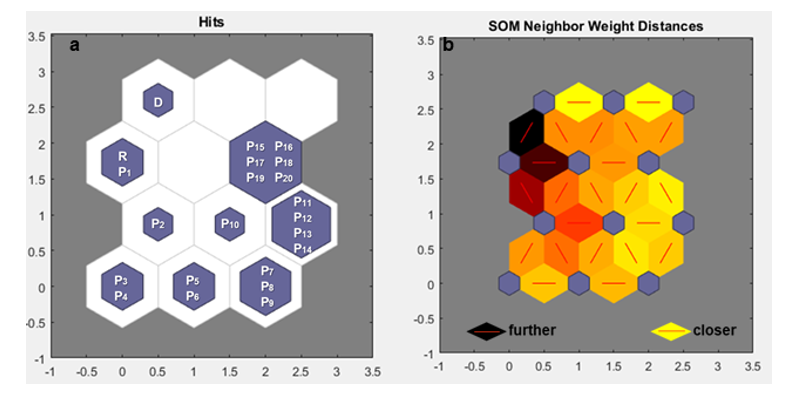

Figure 9: a. Mapping performed by the Self-Organizing Map (SOM) under the effect of migration, with the value of m = 300 for 20 generations, on a 4X3 neuron matrix (row X column). b. Mapping of distance between neurons, based on coloring by SOM under the effect of migration, with the value of m = 300 for 20 generations, on a 4X3 neuron matrix (row X column). Donor base population (D); Receptor base population (R); Subpopulations (P1, P2, P3,...)
 

Several studies have shown Artificial Neural Networks (ANNs) to be quite promising as an efficient alternative for the selection of divergent genotypes in Carica papaya L, for classification studies of alfalfa genotypes, in the evaluation of genetic resources in germplasm databases, in studies on genetic diversity among biomass sorghum (Sorghum bicolor) genotypes, to distinguish dissimilarity among colored fiber cotton genotypes, and in identifying genetic similarities among BC1F3 dwarf tomato populations, among others [10-14].

SOMs have proven to be more efficient in highlighting genetic diversity and grouping populations than traditional methodologies such as the UPGMA method and Tocher's clustering for Nei's GST statistic and Hedrick's Genotypic Measure. This was evident in the identification of genetic similarities among BC1F3 dwarf tomato populations, enabling the determination of the weight of each variable in cluster formation. Additionally, SOM demonstrated greater discriminative capacity among genotypes compared to the UPGMA method. While UPGMA grouped the BC1F3 dwarf populations into two clusters, SOM distributed the populations into ten distinct groups [15].

Fonseca demonstrated the effectiveness of SOMs in highlighting the genetic diversity of populations simulated under divergent selection [7]. Through simulations conducted using the Genes software integrated with Matlab 2016a, the author generated SOMs capable of identifying diversity patterns for both higher selection indices (W1 = ±0.02) and the two lower indices (W2 = ±0.02 and W3 = ±0.002). Additionally, the author noted that traditional methodologies - such as Tocher's clustering for Nei's statistics and Hedrick's Genotypic Measure - were also able to group subpopulations with higher genetic diversity. However, they faced greater challenges with lower index values and had limitations in representing the degree of proximity between these groups and how these subpopulations relate to each other. Both the results obtained by SOMs and the results of the traditional methodologies described by Fonseca exhibited a similar pattern to the findings in this study [7]. In other words, Nei's GST statistic and Hedrick's Genotypic Measure clustered by Tocher were able to detect genetic variability between generations. However, they couldn't reveal what occurred as more migrants arrived over generations. On the other hand, SOMs provided a more prominent representation of how each generation behaved and what changes occurred between generations as more migrants arrived.

What becomes more evident from the results of Fonseca et al. and this study is the ability of SOMs to illustrate the relationships among populations, even under conditions of lower genetic diversity [7]. In contrast, conventional techniques, by not revealing the relationships between populations within the same group and the proximity between groups, fail to highlight small changes that occur over one or a few generations.

Conclusion

The traditional methodologies - Tocher's Clustering for Nei's GST Statistics and Hedrick's Genotypic Measure - were able to group subpopulations with higher diversity; however, they faced difficulties with lower values. On the other hand, Self-Organizing Maps (SOMs) proved capable of organizing populations subjected to processes that increase genetic variability (migration) and also showed the relationship between populations. It is possible to observe, through these results, that migration reduces the differences between populations over time if there is no arrival of new migrants, even under conditions where the numbers of migrants and generations subjected to migration are smaller [16- 18].

Acknowledgement

The authors would like to thank the Research Productivity Scholarship Program (PQ - UEMG) and Institutional Program for Research Support (PAPq) - UEMG, for the financial support. We also appreciate Erik Vinicius Amaro Alves, a student of the Mathematics Course at the University of the State of Minas Gerais (UEMG), for translating the article from Portuguese to English.

References

1. da Silva Oliveira, M., dos Santos, I. G., & Cruz, C. D. (2020). Self-organizing maps: a powerful tool for capturing genetic diversity patterns of populations. Euphytica, 216(3), 49.
2. Frankham, R., Gilligan, D. M., Morris, D., & Briscoe,D.  A.  (2001).  Inbreeding  and  extinction:  effects  of purging. Conservation Genetics, 2, 279-284.
3. Salman, A. K. D. (2007). Conceitos básicos de genética depopulações.
4. Santos, I. G. D., Carneiro, V. Q., Silva, A. C. D., Cruz, C. D., & Soares, P. C. (2018). Self-organizing maps in the study of genetic diversity among irrigated rice genotypes. Acta Scientiarum. Agronomy, 41, e39803.
5. Ibrahim, O. M., Tawfik Elh, M. M., Badr, A., & Wali, A. M. (2016). Evaluating the performance of 16 Egyptian wheat varieties using self-organizing map (SOM) and cluster analysis. Journal of Applied Sciences, 16(2), 47-53.
6. Cruz, CD, Ferreira, FM, & Pessoni, LA (2011). Biometrics applied to the study of genetic diversity. Visconde do Rio Branco: Suprema , 620.
7. Fonseca VPG (2021) Diferenciação genética em populações simuladas sob seleção divergente utilizando mapas auto- organizáveis. Dissertação, Universidade do Estado de Minas Gerais, Carangola.
8. Cruz, C. D. (2013). Genes: a software package for analysis in experimental statistics and quantitative genetics. Acta Scientiarum. Agronomy, 35, 271-276.
9. Cruz, C. D. (2016). Genes Software-extended and integrated with the R, Matlab and Selegen. Acta Scientiarum. Agronomy, 38(4), 547-552.
10. Barbosa, C. D., Viana, A. P., Quintal, S. S. R., & Pereira,M. G. (2011). Artificial neural network analysis of genetic diversity in Carica papaya L. Crop Breeding and Applied Biotechnology, 11, 224-231.
11. Santos, I. G., Cruz, C. D., Nascimento, M., & Ferreira, R. D.P. (2019). Selection index as a priori information for using artificial neural networks to classify alfalfa genotypes.
12. Moura MCCL et al. (2015). Potencialidades das redes neurais artificiais na avaliação de recursos genéticos em bancos de germoplasma. Revista RG News: Sociedade Brasileira de Recursos Genéticos, 1:14-19.
13. da Silva, M. J., da Silva Júnior, A. C., Cruz, C. D., Nascimento, M., da Silva Oliveira, M., Schaffert, R. E., & da Costa Parrella, R. A. (2020). Inteligência computacional para estudos de diversidade genética entre genótipos de sorgo biomassa. Pesquisa Agropecuária Brasileira, 55(X), 01723.
14. Pimentel, IM (2021). Use of artificial neural networks in the evaluation of the dissimilarity of colored fiber cotton.
15. de Oliveira, C. S., Maciel, G. M., Siquieroli, A. C. S., Gomes, D. A., Diniz, N. M., Luz, J. M. Q., & Yada, R. Y. (2021). Artificial neural networks and genetic dissimilarity among saladette type dwarf tomato plant populations. Food Chemistry: Molecular Sciences, 3, 100056.
16. Golgher, A. B. (2004). Fundamentos da migração. Belo Horizonte: UFMG/Cedeplar, (231).
17. Leichtweis, BG (2021). Self-organizing Kohonen maps for environmental clustering and study of genotype-by- environment interactions via reaction norms.
18. Sudheer, K. P., Gosain, A. K., & Ramasastri, K. S. (2003). Estimating actual evapotranspiration from limited climatic data using neural computing technique. Journal of irrigation and drainage engineering, 129(3), 214-218.