Are Some Voltage State Orbits, Computed in a Discrete-Time Hopfield Neural Network, Which Correspond to Bifurcation Values, Fractals? Exists these Orbits in Reality or they Exists Just in Theory i.e. has these Orbits a Real Counterpart?

Introduction

There is some disagreement among mathematician about how the concept of fractal should be formally defined. Mandelbrot himself summarized it is as “beautiful damn hard increasingly useful. That’s fractals. More formally, in 1982Mandelbrot defined fractal as follows: "A fractal is by definition a set for which the Hausdorff–Besicovitch dimension strictly exceeds the topological dimension [1]."Later, seeing this as too restrictive, he simplified and expanded the definition to this: "A fractal is a rough or fragmented geometric shape that can be split into parts, each of which is (at least approximately) a reduced-size copy of the whole [2]."Still later, Mandelbrot proposed, "to use fractal without a pedantic definition, to use fractal dimension as a generic term applicable to all the variants"[1]. The consensus among mathematicians is that theoretical fractals are infinitely self-similar iterated and detailed mathematical constructs, of which many examples have been formulated and studied [1- 3]. Fractals are not limited to geometric patterns, but can also describe processes in time [4-9]. Fractal patterns with various degrees of self-similarity have been rendered or studied in visual physical, and aural media and found in nature, technology, art, and architecture [10-19]. In this context fractal geometry lies within the mathematical branch of measure theory presenting different measures and algorithms for the computation of different types of fractal dimensions of geometrical patterns; box counting dimension, correlation dimension ,generalized or Renyi dimensions, Higuchi dimension, Lyapunov dimension, Multifractal dimensions, Hausdorff dimension, Packing dimension, Assouad dimension, Local connected dimension, Degree dimension, Parabolic Hausdorff dimension [3,20]. These fractal dimensions strictly exceed the topological dimension and although for compact sets with exact affine self-similarity all these dimensions coincide; in general, they are not equivalent. When fractal describe processes in time, then for the analysis of statistical data, fractal analysis use also tools for: investigate statistical self-similarity, find probability density function (PDF), fractal scaling in time, time series analysis, fractal kinetic description ,power law and fractal statistics. Beside the mathematical description of the voltage dynamics of neural cells and systems using fractals, there exist a large amounts of papers, which use classical theory of electrical circuits or fractional order derivative circuits for describe the neural cells dynamics [4-9,16,21-33]. Papers use classical theory of electricity (integer order differential equations) for the description of the ion transport through the nervous cell membrane [34-41]. Papers use time fractional order circuits for the description of the ion transport through the nervous cell membrane [42-44]. In the papers it was shown that: Mathematical descriptions of the ion transport, across passive or active biological neuron membrane, voltage propagation along neuron axons and dendrites having passive or active membrane and ion transport in biological neuron networks, using classic Caputo or Riemann-Liouville fractional order derivatives, is nonobjective [45,46]. The no objectivity is originated in the incompatibility of the classic Caputo and Riemann- Liouville fractional order derivatives with the understanding of the time evolution, used in case of the mathematical description of real word phenomena.

Hopfield paper claims to be mathematical descriptions of electrical phenomena appearing in nervous system [47]. Later in this model was extended to optimization and cryptography [48–50]. In papers, theoretical studies of the Hopfield neural system are carried out in the continuous time and discrete time versions [51-71]. Papers reveal configuration of steady states, local exponential stability of steady states in Lyapunov sense, regions of attraction of exponential stable steady states, bifurcation properties etc. Several example of low dimensional (two, fife neurons) neural network are presented which exhibit extremely interesting orbits and bifurcation diagrams. Although for some values of the bifurcation parameter the orbits completely disintegrate and no longer resemble what we call orbit in classical sense, their fractal quality is not analyzed and highlighted. In addition, no reference is made to the question: whether or not these completely dismembered orbits have a real counterpart? In the case of strange bifurcation diagrams, their approach with fractals, as far as we know, is not done. In this paper, we will present in case of four neural networks, examples of strange orbits and bifurcation diagrams, and try to bring arguments to support that they are fractals. We also hypothesize that they have a real counterpart. They exists not only in theory.

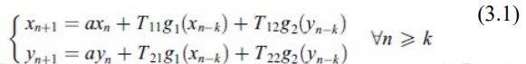
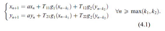
Case of a Discrete-Time Hopfield Neural Network of Two Neurons with Two Delays and No Self- Connections

In an extended analysis of the chaotic dynamics of the neural network defined

was undertaken [67]. The external inputs are equal to zero and the system parameters are regarded as numerical expression of the state of network. The network state can change due to a disease for example. Therefore, the network voltage dynamics change too. In this kind of change is analyzed with respect to the product of the interconnection coefficients as aggregated characteristic parameter for the system [67]. The main result obtained in, is that, if the magnitudes of the interconnection coefficients are large enough, then the neural network exhibits Marotto’s chaotic behavior [67]. For illustrate what this means the following numerical example was considered: a₁ = 1/4, a₂ = 3/4, T₁₂ = 1, g₁(t) = tanh(t) and g₂(t) = sin(t), b = T₂₁ k₁ = 1 and k₂ = 2. For different values of b, trajectory of the neuron’s voltages were computed and represented. We will present some of these trajectories.

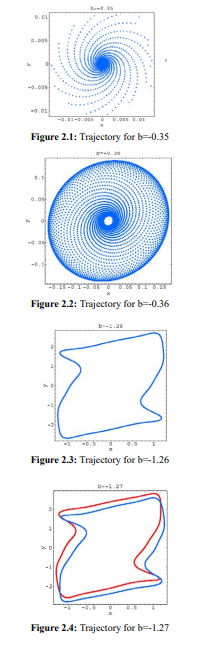
For b=−0.35, the null solution is asymptotically stable, and the trajectories converges to the origin. For b=−0.36, an asymptotically stable cycle (1-torus, drift ring) is present, and the trajectories converges to this cycle. At b = b1 =−0.35635 a supercritical Neimark–Sacker bifurcation takes place. For b = −1.26, there is only one asymptotically stable limit cycle (1-torus), symmetrical to the origin. For b =−1.27, there are two stable limit cycles, not symmetrical to the origin. For each plot, the first 106 iterations have been dropped, and the next 104 iterations have been plotted. At around b =−1.265, a bifurcation phenomenon takes place, which determines the appearance of two stable limit cycles (1-tori) close to the origin.

For the localization of bifurcations values the Largest Lyapunov Characteristic Exponent (LCE) and the Lyapunov spectrum (LCEs) for system (2.1) was used. For the computation of the Lyapunov spectrum, for each b value (step size 0.01 for b), the initial conditions were reset and 105 time-steps were iterated before calculating the LCEs (which were computed over the next 105 time steps). The Lyapunov spectrum was computed using the Householder QR based (HQRB) method. The obtained LCE and LCEs are represented in Fig.2.5. and Fig.2.6. respectively.

Figure 2.5: Largest Lyapunov Characteristic Exponent

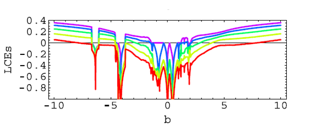
Figure 2.6: Largest Lyapunov Characteristic Spectrum

The trajectories presented in Fig. 2.1-Fig.2.4 are what we call orbits in classical sense. However, they become more and more complex for various values of b ∈ (−1.5, −1.4). This can be seen on the following figures.

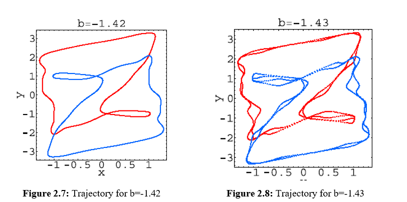
Figure 2.7: Trajectory for b=-1.42                             Figure 2.8: Trajectory for b=-1.43

Figure 2.9: Trajectory for b=-1.457                               Figure 2.10: Trajectory for b=-1.46

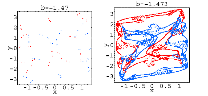
Figure 2.11: Trajectory for b=-1.47                                Figure 2.12: Trajectory for b=-1.473

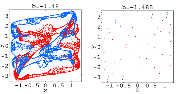
Figure 2.13: Trajectory for b=-1.48                               Figure 2.14: Trajectory for b=-1.485

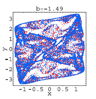
Figure 2.15: Trajectory for b=-1.49

Hear for each plot, the first 106 iterations of system (2.1) have been dropped, and the next 104 iterations have been plotted. These trajectories corresponds to the bifurcations values: b=−1.42: 1-tori; b=−1.43: 2-tori; b=−1.457: 2-tori declining into strange attractors; b =−1.46: strange attractors; b =−1.47: two stable period-52 orbits; b =−1.473: strange attractors; b =−1.48: strange attractors; b =−1.485: two stable period-39 orbits; b=−1.49: strange attractors.

It seems that from bifurcation point of view, everything is clear but from the point of view of the trajectory, geometry is not at all clear. That is because it can be seen that “Trajectories” presented in Fig.2.10.-Fig.2.15. are not at all what we call orbits in classic sense. Their geometry moreover is fractal. Are “Trajectories” presented in Fig.2.10.-Fig.2.15 objects of Fractal Geometry? Have they real counterpart or they exist just in theory? There are similar behavior mentioned in or elsewhere in specialized literature? These are our main questions. In our opinion Fig.2.10- Fig.2.15. are fractals. If not, what are these geometrical figures [10,12,16,21-25,27-33]?

For various values of b ∈ (−10,−2) the trajectories were also computed using the same procedure i.e. the first 106 Iterations of system (2.1) have been dropped, and the next 104 iterations have been plotted.

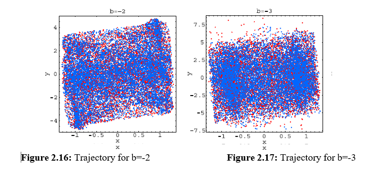
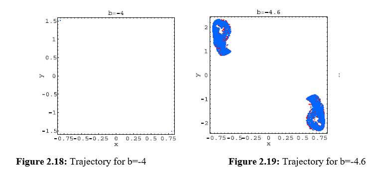
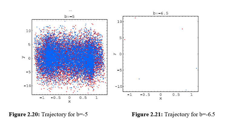
Figure 2.22: Trajectory for b=-7                                    Figure 2.23: Trajectory for b=-9

These trajectories corresponds to the bifurcation’s values: b =−2: hyperchaos (LE2 > 0, LE3 < 0) b=−3: hyperchaos (LE3 > 0, LE4 < 0); b=−4: one stable period-2 orbit (LE1 < 0); b=−4.6: strange attractor developing from the period-2 solution; b = −5: hyperchaos (LE4 > 0, LE5 < 0); b = −6.5: two stable period-3 orbits (LE1 < 0); b = −7: hyperchaos (LE4 > 0, LE5 < 0); b = −9: hyperchaos (LE5 > 0).

Our main questions are the same: are “Trajectories” presented in Fig.2.16.-Fig.2.23 objects of Fractal Geometry? Have they real counterpart or they exist just in theory? If not, what are these geometrical figures? There are similar behavior mentioned in [10-12,16,21-25,27-33] or elsewhere in specialized literature? Our conjecture is that ‘Trajectories” presented in Figs:2.10.- 2.23.are fractals and has real counterpart.

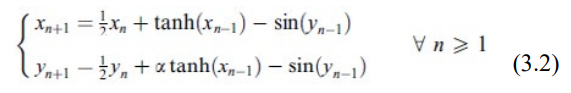
Case of a Discrete-Time Hopfield Neural Network of Two Neurons with a Single Delay and Self- Connections

In an analysis of the dynamics of the neural network defined by

was undertaken [68]. The external inputs are equal to zero and the system parameters are regarded as numerical expression of the state of network. The network state can change due to a disease for example. Therefore, the network voltage dynamics change too. In this kind of change is analyzed [68].The conclusion in, is: The bifurcation analysis of two-dimensional discrete- time Hopfield neural networks with a single delay reveals the existence of Neimark–Sacker, fold and some codimension 2 bifurcations values of the bifurcation parameters that have been chosen [68]. For illustrate what this means the following numerical example was considered:

The origin is asymptotically stable if and only if At 1.40693 a supercritical Neimark–Sacker bifurcation occurs.

          Fig.3.1. Trajectory for @=1.4                                       Fig.3.2. Trajectory for

Figure 3.3: Trajectory for α=1.5

For α=1.4, the null solution of (3.2) is asymptotically stable. Fig.3.1.illustrate that the trajectories of (3.2) converges to the null solution. These trajectories are what we call orbits in classic sense. For α=1.5, the null solution is unstable and an asymptotically stable closed invariant curve is present. The trajectory of (3.2) converges to the asymptotically stable invariant curve as is shown in Fig.3.2. Fig.3.3.The trajectories presented in Fig. 3.2, Fig.3.3 are what we call orbits in classical sense. This summary analysis does not reveal trajectories that are no longer classic curves. Even the asymptotically stable closed invariant curve, corresponding to the bifurcation value α=1.5, is a classical curve.

Case of a Discrete-Time Hopfield Neural Network of Two Neurons with a Two Delays and Self- Connections

In an analysis of the dynamics of the neural network defined by

is undertaken [69]. The external inputs are equal to zero and the system parameters are regarded as numerical expression of the state of network. The network state can change due to a disease for example. Therefore, the network voltage dynamics change too. In this kind of change is analyzed [69]. The conclusion in, is: “The results presented in this paper complete the bifurcation results obtained for discrete-time Hopfield neural networks with a single delay and self-connections presented in and for networks with two delays and no self-connections presented in, with new results concerning the case of neural networks with two different delays and self-connections, revealing some resemblances (the existence of Neimark-Sacker, Fold, resonance 1:1, double Neimark-Sacker bifurcations) and some differences (the possible existence of Flip and Flip–Neimark-Sacker bifurcations), as well” [66,68,69]. For illustrate what this means the following numerical example was considered:

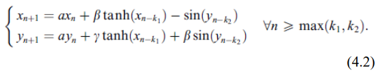
with; a = 0.5, k1 = 4, k2 = 10,

For γ=0.19 the null solution of (4.2) is asymptotically stable and trajectories converges to the null solution.Fig.4.1.illustrate that the trajectories of (4.2) converges to the null solution and the fact that these trajectories are what we call orbits in classic sense.

For γ=0.2 the null solution is unstable and an asymptotically stable closed invariant curve is present. The trajectories of (4.2) converges to the asymptotically stable invariant curve as is shown in Fig.4.2., Fig.4.3. The trajectories presented in Fig. 4.2, Fig.4.3 are what we call orbits in classical sense.

For β=0.82 and γ=0.47 the null solution of (4.2) is unstable and an asymptotically stable cycle of period 2 is present. The trajectory of (4.2) converges to the asymptotically stable cycle i.e. Flip (period-doubling) bifurcation occurs as is shown in Fig.4.4.. The trajectory presented in Fig. 4.4, are what we call orbit in classical sense.

This summary analysis does not reveal trajectories that are no longer classic curves.

Figure 4.1: Trajectory for γ=1.19

 Figure 4.2: Trajectory for γ = 0.2                          Figure 4.3: Trajectory for γ = 0.2

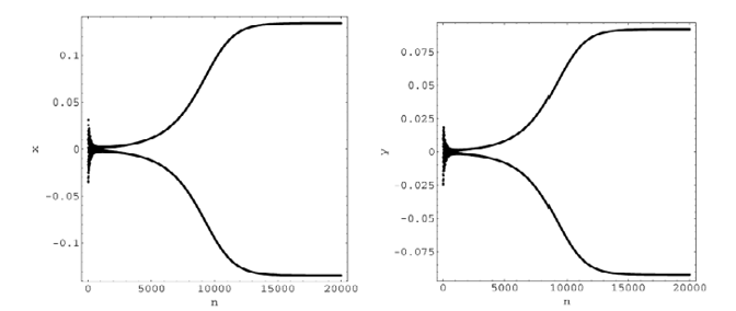
Figure 4.4: Trajectory for β = -0.82, γ = -0.47

Case of a Discrete-Time Hopfield Neural Network with Delay and Ring Architecture

In an extended analysis of the chaotic dynamics of the neural network with delay and ring architecture defined by

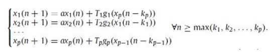
was undertaken [70]. The external inputs are equal to zero and the system parameters are regarded as numerical expression of the state of network. The network state can change due to a disease for example. Therefore, the network voltage dynamics change too. In this kind of change is analyzed with respect to the network parameters [70]. The stability domain of the null solution is found, the values of the characteristic parameter for which bifurcations occur at the origin are identified and the existence of Fold/Cusp, Neimark-Sacker and Flip bifurcations is proved. These bifurcations were analyzed by applying the center manifold theorem and the normal form theory. It is proved that resonant 1:3 and 1:4 bifurcations may be present. It is shown that the dynamics in a neighborhood of the null solution become more and more complex as the characteristic parameter grows in magnitude and passes through the bifurcation values. A theoretical proof is given for the occurrence of Marotto's chaotic behavior, if the magnitudes of the interconnection coefficients are large enough and at least one of the activation functions has two simple real roots. For illustrate what this means the following numerical example was considered:

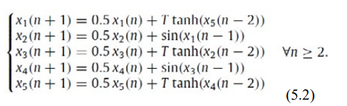
All numerical computations have been done using Mathematica. Denoting b=T3, based on the theoretical result presented, we find that the critical values of b are {-7.593;-6.396;-3.784; -1.538; -0.433; -0.102; -0.036; 0.031; 0.055; 0.209;0.851; 2.531; 5.148; 7.276}. The stability domain of the null solution, with respect to T is DS= (-0.331116; 0.31498). At T= 0.31498, a Cusp bifurcation occurs at the origin, while at T=-0.331116 a supercritical Neimark-Sacker bifurcation takes place (as shown in Fig.5.1)

         Figure 5.1: Supercritical Neimark-Sacker bifurcation at T=-0.331116

For T=-0.33, the null solution is asymptotically stable, and the trajectory converges to the origin. For T=-0-34, an asymptotically stable cycle (1-torus, drift ring) is present, and the trajectory converges to this cycle. If modulus T is sufficiently large, chaotic behavior may be expected. Figs. 5.1-5.4 describe the route towards chaos occurring in system (5.2) in a neighborhood of the origin, as T decreases from 0 to -3. The bifurcation diagram (Fig. 5.2) and the computed four largest Lyapunov Characteristic Exponents shown in Fig. 5.3, (computed using the Householder QR based method developed by Bremen, Udwadia, and Proskurowski (1997)), clearly describe this route, being consistent with the theoretical results presented.

Figure 5.2: Bifurcation Diagram for System (5.2), in the (T, x1) -Plane, for -3< T<0, with the Step Size of 0:005 for T

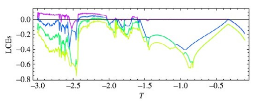
Figure 5.3: Four Largest Lyapunov Characteristic Exponents for System (5.2)

For the computation of the Lyapunov spectrum, for each T value (step size 0:005 for T) the initial conditions were reset and 105 time steps were iterated before calculating the LCEs (which were computed over the next 105 time steps). In Fig.5.4. Phase portraits for various values of T, -3

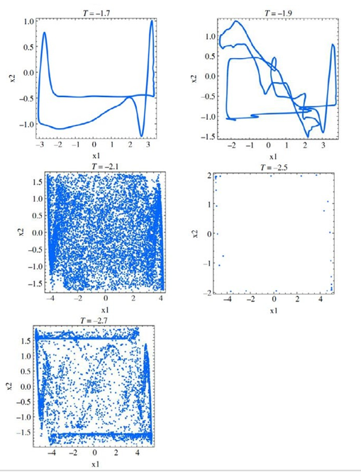
Figure 5.4: Phase Portraits for: T=-1.4; T=-1.45; T=-1.5; T=-1.65; T=-1.7; T=-1.9; T=-2.1; T=-2.5; T=-2.7

From the bifurcation point of view, the meaning of these figures is clear: T=-1.4, stable torus (LE1= 0); T=-1.45, stable period-32 orbit (LE1 < 0); T=-1.5, stable torus (LE1= 0); T=1.65, chaos (LE1 > 0); T=-1.7; T =-1.9, stable tori (LE1= 0);T =-2.1, hyperchaos (LE3 > 0); T=-2.5, stable period-38 orbit (LE1 < 0); T=-2.7, chaos (LE1 > 0). The question is: are the phase portrait corresponding to T=-1.45, T=-1.65, T=-2.1, T= -2.5, T=--2.7 objects of Fractal Geometry? Have they real corresponding or they exist just in theory? Our conjecture, based on the geometrical aspect, is that the phase portraits for T=-1.45, T=-1.65, T=-2.1, T=_2.5, T=-- 2.7 are fractals and they have real counterpart.

Results

In case of a discrete-time Hopfield neural network of two neurons with two delays and no self- connections 23 voltage “trajectories” are computed at bifurcation points. Among the 23 voltage “trajectories” we find 14 voltage trajectory which are not what we can call orbits in classic sense. The geometrical aspect of these trajectories suggest that they are fractals. Our conjecture is that the 14 trajectories in discussion are fractals and has real counterpart.

In case of a discrete-time Hopfield neural network of five neuron with delay and ring architecture 9 voltage “trajectories” appear at bifurcation points. Among the 9 voltage trajectories we find 5 voltage “trajectory” which are not what we can call “orbits” in classic sense. The geometrical aspect of these “trajectories” suggest that they are fractals. Our conjecture is that the 5 trajectories in discussion are fractals having real counterpart.

Discussion

The scientific literature concerning fractals in the description of nervous system is extensive.

In for example it is shown that, Currents through Ion Channels has fractal properties in time, Electrical Activity of Auditory Nerve Cells is described in terms of fractal [21].

In authors sustain that “fractal and conventional morphometry may represent complementary analytical/ quantitative tools to elucidate the diversity of morphological patterns and functional parameters which characterize neural cells and brain structures” [22].

In the author writ: “the present survey provides experimental data confirming that biological processes including growth, proliferation, apoptosis, epigenetic and genetic mechanism, morphologic/ultrastructural and functional organization occurring in living shaped elements and complex structured tissues may follow fractal rules [23]. The large agreement with the fractal nature of the brain and nervous cell system sustained by theoretical, experimental and heuristic foundations is nowadays consolidated and intervenes more than thirty years after the publication of the Fractal Geometry of Nature, in which Mandelbrot recognized that “the notion that neurons are fractals remains conjectural” Its relevance and contribution to the cultural development of mankind (as comprehensive of humanistic and scientific thinking) is keen underlined by the observation of some years ago arguing that the fractal geometry could be considered as a biological design principle for living organisms.

Paper use fractal time series analysis (detrended fluctuation analysis; DFA) to examine the spontaneous activity of single neurons in an anesthetized animal model, specifically, the mitral cells in the rat main olfactory bulb [24]. DFA bolstered previous research in suggesting two subclasses of mitral cells. Although there was no difference in the fractal scaling of the interspike interval series at the shorter timescales, there was a significant difference at longer timescales. Neurons in Group B exhibited fractal, power-law scaled interspike intervals, whereas neurons in Group A exhibited random variation. These results raise questions about the role of these different cells within the olfactory bulb and potential explanations of their dynamics. Specifically, self-organized criticality has been proposed as an explanation of fractal scaling in many natural systems, including neural systems. However, this theory is based on certain assumptions that do not clearly hold in the case of spontaneous neural activity, which likely reflects intrinsic cell dynamics rather than activity driven by external stimulation. Moreover, it is unclear how self-organized criticality might account for the random dynamics observed in Group A, and how these random dynamics might serve some functional role when embedded in the typical activity of the olfactory bulb.

In the paper the authors conclude:” Given the central role of brain’s “wiring”, our previous research for focused on the importance of fractal scaling in establishing connectivity between neurons [25]. Diagnostic Analysis (DA} was show to relate to the optimization of competing functional constraints—the ability of dendrites to reach out and connect other neurons versus the costs associated with doing so. Within this model, different neuron types were predicted to different DA values depending on the relative importance of connectivity and material cost with higher DA values indicating a greater emphasis on connectivity. In the current investigation, we hypothesize that pathological state of neurons might also affect this fractal optimization and consider whether changes in DA might therefore, be used as a diagnostic tool. This analysis represents an appealing development because it relates form to function rather than relying purely on pattern characterization.”

Our approach in this paper is different from those presented in the above-referred literature. We start considering the discrete- time Hopfield neural network model, which claim to describe the electrical activity of a neural system. The bifurcation analysis of some low dimensional networks show that for certain values of the bifurcation parameter the geometry of the voltage orbits of neurons are what we call classic orbits and there exists other bifurcation values for which the geometrical aspect of trajectories are not at all what we call classic orbits. Their geometrical aspects suggest that they are moreover fractals. The present paper present to the reader both type of trajectories putting the natural question: Are some of the presented voltage state orbits, fractals? Exists these orbits in reality or they exists just in theory i.e. has these orbits a real counterpart? Our conjecture is that some of the voltage trajectories presented here are fractals and have real counterpart.

Author Contributions

The two authors contributed equally to the realization of this work. All authors have read and agreed to the published version of the manuscript.

References

1. Mandelbrot, Benoit (July 8, 2013). "24/7 Lecture on Fractals"
2. https://ghostarchive.org/varchive/youtube/20211211/5e7H- B5Oze4g) from the original on December 11, 2021.
3. Mandelbrot, B. B. (1982). TheFractalGeometryofNature.WH Freedman and Co., New York, 1(983), 1.
4. Edgar, Gerald (2007). Measure, Topology, and Fractal Geometry.
5. Vicsek, T. (1992). Fractal growth phenomena. World scientific.
6. Gouyet, Jean-François (1996). Physics and fractal structures. Paris/New York: Masson Springer. ISBN 978- 0-387-94153-0.
7. Peters, E. E. (1996). Chaos and order in the capital markets: a new view of cycles, prices, and market volatility. John Wiley & Sons.
8. Krapivsky, P. L., & Ben-Naim, E. (1994). Multiscaling in stochastic fractals. Physics Letters A, 196(1-2), 168-172.
9. Hassan, M. K.; Rodgers, G. J. (1995). "Models of fragmentation and stochastic fractals". Physics Letters A. 208 (1–2): 95. Bibcode:1995PhLA..208...95H
10. Hassan, M. K., Pavel, N. I., Pandit, R. K., & Kurths, J. (2014). Dyadic Cantor set and its kinetic and stochastic counterpart. Chaos, Solitons & Fractals, 60, 31-39.
11. Tan, C. O., Cohen, M. A., Eckberg, D. L., & Taylor, J. A. (2009). Fractal properties of human heart period variability: physiological and methodological implications. The Journal of physiology, 587(15), 3929-3941.
12. Liu, J. Z., Zhang, L. D., & Yue, G. H. (2003). Fractal dimension in human cerebellum measured by magnetic resonance imaging. Biophysical journal, 85(6), 4041-4046.
13. Karperien, A. L., Jelinek, H. F., & Buchan, A. M. (2008). Box-counting analysis of microglia form in schizophrenia, Alzheimer's disease and affective disorder. Fractals, 16(02), 103-107.
14. Jelinek, H., Karperien, A., Cornforth, D., Cesar, R. M. J., & Leandro, J. (2002, November). MicroMod—an L-systems approach to neuron modelling. In Proceedings of the Sixth Australasia-Japan Joint Workshop on Intelligent and Evolutionary Systems, Australian National University, Canberra (pp. 156-163).
15. Hu, S., Cheng, Q., Wang, L., & Xie, S. (2012). Multifractal characterization of urban residential land price in space and time. Applied Geography, 34, 161-170.
16. Karperien, Audrey; Jelinek, Herbert F.; Leandro, Jorge de Jesus Gomes; Soares, João V. B.;Cesar Jr, Roberto M.; Luckie, Alan. (2008). "Automated detection of proliferative retinopathy in clinical practice". Clinical Ophthalmology. 2(1): 109–122.
17. Losa, Gabriele A.; Nonnenmacher, Theo F. (2005). Fractals in biology and medicine. Springer. ISBN 978-3-7643-7172- 2.
18. Vannucchi, P., & Leoni, L. (2007). Structural characterization of the Costa Rica décollement: Evidence for seismically- induced fluid pulsing. Earth and Planetary Science Letters, 262(3-4), 413-428.
19. Wallace, David Foster (August 4, 2006). "Bookworm on KCRW". Kcrw.com. Archived from the original (http:// www.kcrw.com/etc/programs/bw/bw960411david_foster_ wallace) on November 11, 2010. Retrieved October 17,2010)
20. Eglash, R. (1999). African fractals: Modern computing andindigenous design.
21. New Brunswick: Rutgers University Press. Archived from the original on January 3, 2018. Retrieved October 17,2010.
22. Ostwald, M. J., & Vaughan, J. (2016). The fractal dimension of architecture (Vol. 1). Birkhäuser.
23. Liebovitch, L. S. (1998). Fractals and chaos simplified forthe life sciences.
24. Losa, G. A., Di Ieva, A., Grizzi, F., & De Vico, G. (2011). On the fractal nature of nervous cell system. Frontiers in Neuroanatomy, 5, 45.
25. Losa, G. A. (2014). On the fractal design in human brain and nervous tissue. Applied mathematics, 2014.
26. Favela, L. H., Coey, C. A., Griff, E. R., & Richardson, M.J. (2016). Fractal analysis reveals subclasses of neurons and suggests an explanation of their spontaneous activity. Neuroscience letters, 626, 54-58.
27. Rowland, C., Harland, B., Smith, J. H., Moslehi, S., Dalrymple-Alford, J., & Taylor, R. P. (2022). Investigating fractal analysis as a diagnostic tool that probes the connectivity of hippocampal neurons. Frontiers in Physiology, 13, 932598.
28. Pilgrim, I., & Taylor, R. P. (2018). Fractal analysis of time- series data sets: Methods and challenges. Fractal analysis, 5-30.
29. Zaletel, I. V., & Puškaš, N. (2016). Fractal analysis in neuroanatomy and neurohistology. Medicinski podmladak, 67(4).
30. Wonsang You, Sophie Achardy, J¨org Stadler, Bernd Bruckner, and Udo Seiffert, Fractal analysis of resting state functional connectivity of the brain, WCCI 2012 IEEE World Congress on Computational Intelligence, June, 10- 15, 2012 - Brisbane, Australia
31. Teich, M. C., Heneghan, C., Lowen, S. B., Ozaki, T., & Kaplan, E. (1997). Fractal character of the neural spike train in the visual system of the cat. JOSA A, 14(3), 529-546.
32. Di Ieva, A., Grizzi, F., Jelinek, H., Pellionisz, A. J., & Losa,G. A. (2014). Fractals in the neurosciences, part I: general principles and basic neurosciences. The Neuroscientist, 20(4), 403-417.
33. Di Ieva, A., Esteban, F. J., Grizzi, F., Klonowski, W., & Martín-Landrove, M. (2015). Fractals in the neurosciences, part II: clinical applications and future perspectives. The Neuroscientist, 21(1), 30-43.
34. Gerhard Werner, Fractals in the nervous system: conceptual implications for theoretical neuroscience, Frontiers in Physiology | Fractal Physiology, July 2010 | Volume 1 | Article 15.
35. Bieberich, E. (2002). Recurrent fractal neural networks: a strategy for the exchange of local and global information processing in the brain. Biosystems, 66(3), 145-164.
36. Hodgkin, A. L., & Huxley, A. F. (1952). A quantitative description of membrane current and its application to conduction and excitation in nerve. The Journal of physiology, 117(4), 500.
37. Hagiwara, S., & Nakajima, S. (1966). Effects of the intracellular Ca ion concentration upon the excitability of the muscle fiber membrane of a barnacle. The Journal of general physiology, 49(4), 807-818.
38. Hagiwara, S., Hayashi, H., & Takahashi, K. (1969). Calcium and potassium currents of the membrane of a barnacle muscle fibre in relation to the calcium spike. The Journal of physiology, 205(1), 115-129.
39. Keynes, R. D., Rojas, E., Taylor, R. E., & Vergara, J. (1973). Calcium and potassium systems of a giant barnacle muscle fibre under membrane potential control. The Journal of physiology, 229(2), 409.
40. Hagiwara, S., Fukuda, J., & Eaton, D. C. (1974). Membrane currents carried by Ca, Sr, and Ba in barnacle muscle fiber during voltage clamp. The Journal of general physiology, 63(5), 564-578.
41. Murayama, K., & Lakshminarayanaiah, N. (1977). Some electrical properties of the membrane of the barnacle muscle fibers under internal perfusion. The Journal of Membrane Biology, 35(1), 257-283.
42. Beirao, P. S., & Lakshminarayanaiah, N. (1979). Calcium carrying system in the giant muscle fibre of the barnacle species, Balanus nubilus. The Journal of Physiology, 293(1), 319-327.
43. Morris, C., & Lecar, H. (1981). Voltage oscillations in the barnacle giant muscle fiber. Biophysical journal, 35(1), 193-213.
44. Weinberg, S. H. (2015). Membrane capacitive memory alters spiking in neurons described by the fractional-order Hodgkin-Huxley model. PloS one, 10(5), e0126629.4
45. Brandibur, O., & Kaslik, E. (2017). Stability properties of a two-dimensional system involving one Caputo derivative and applications to the investigation of a fractional-order Morris–Lecar neuronal model. Nonlinear Dynamics, 90(4), 2371-2386.
46. Moreles, M. A., & Lainez, R. (2016). Mathematical modelling of fractional order circuits. arXiv preprint arXiv:1602.03541.
47. Balint, A. M., Balint, Ã…?., & Szabo, R. (2021). Mathematical description of the ion transport across biological neuron membrane and in biological neuron networks, voltage propagation along neuron axons and dendrites, which uses temporal classic Caputo or Riemann-Liouville fractional partial derivatives, is non-objective. Mathematics in Engineering, Science & Aerospace (MESA), 12(4).
48. Balint, A. M., Balint, S., & Neculae, A. (2022). On the objectivity of mathematical description of ion transport processes using general temporal Caputo and Riemann- Liouville fractional partial derivatives. Chaos, Solitons & Fractals, 156, 111802.
49. Hopfield, J. J. (1982). Neural networks and physical systems with emergent collective computational abilities. Proceedings of the national academy of sciences, 79(8), 2554-2558.
50. Tank, D., & Hopfield, J. (1986). Simple'neural'optimization networks: An A/D converter, signal decision circuit, and a linear programming circuit. IEEE transactions on circuits and systems, 33(5), 533-541.
51. Yu, W., & Cao, J. (2006). Cryptography based on delayed chaotic neural networks. Physics Letters A, 356(4-5), 333- 338.
52. Darau, M., Kaslik, E., & Balint, S. (2012). Cryptography using chaotic discrete-time delayed Hopfield neural networks. Mathematics in Engineering, Science and Aerospace, 3(1), 31-40.
53. Adachi, M., & Aihara, K. (1997). Associative dynamics in a chaotic neural network. Neural Networks, 10(1), 83-98.
54. von Bremen, H. F., Udwadia, F. E., & Proskurowski, W. (1997). An efficient QR based method for the computation of Lyapunov exponents. Physica D: Nonlinear Phenomena, 101(1-2), 1-16.
55. Chen, L., & Aihara, K. (1995). Chaotic simulated annealing by a neural network model with transient chaos. Neural networks, 8(6), 915-930.
56. Chen, L., & Aihara, K. (1997). Chaos and asymptotical stability in discrete-time neural networks. Physica D: Nonlinear Phenomena, 104(3-4), 286-325.
57. Chen, L., & Aihara, K. (2001). Chaotic dynamics of neural networks and its application to combinatorial optimization. Differential Equations and Dynamical Systems, 9(3-4), 139-168.
58. Chen, S. S., & Shih, C. W. (2002). Transversal homoclinic orbits in a transiently chaotic neural network. Chaos: An Interdisciplinary Journal of Nonlinear Science, 12(3), 654- 671.
59. Guo, S., & Huang, L. (2004). Periodic oscillation for discrete-time Hopfield neural networks. Physics Letters A, 329(3), 199-206.
60. Guo, S., Huang, L., & Wang, L. (2004). Exponential stability of discrete-time Hopfield neural networks. Computers & Mathematics with Applications, 47(8-9), 1249-1256.
61. Guo, S., Tang, X., & Huang, L. (2008). Stability and bifurcation in a discrete system of two neurons with delays. Nonlinear Analysis: Real World Applications, 9(4), 1323- 1335.
62. He, W., & Cao, J. (2007). Stability and bifurcation of a class of discrete-time neural networks. Applied Mathematical Modelling, 31(10), 2111-2122.
63. Kaslik, E. (2006). Configurations of steady states for Hopfield-type neural networks. Applied mathematics and computation, 182(1), 934-946.
64. Balint, È?., BrÄ?escu, L., & Kaslik, E. (2008). Regions of attraction and applications to control theory (Vol. 1). Cambridge Scientific Publishers.
65. Yuan, Z., Hu, D., & Huang, L. (2004). Stability and bifurcation analysis on adiscrete-time system of two neurons. Applied mathematics letters, 17(11), 1239-1245.
66. Yuan, Z., Hu, D., & Huang, L. (2005). Stability and bifurcation analysis on a discrete-time neural network. Journal of Computational and Applied Mathematics, 177(1), 89-100.
67. Zhang, C., & Zheng, B. (2005). Hopf bifurcation in numerical approximation of a n-dimension neural network model with multi-delays. Chaos, Solitons & Fractals, 25(1), 129-146.
68. Zhang, C., & Zheng, B. (2007). Stability and bifurcation of a two-dimension discrete neural network model with multi- delays. Chaos, Solitons & Fractals, 31(5), 1232-1242.
69. Kaslik, E., & Balint, Ã…?. (2008). Chaotic dynamics of a delayed discrete-time Hopfield network of two nonidentical neurons with no self-connections. Journal of Nonlinear Science, 18, 415-432.
70. Kaslik, E. (2007). Bifurcation analysis for a two-dimensional delayed discrete-time Hopfield neural network. Chaos, Solitons & Fractals, 34(4), 1245-1253.
71. Kaslik, E. (2009). Bifurcation analysis for a discrete-time Hopfield neural network of two neurons with two delays and self-connections. Chaos, Solitons & Fractals, 39(1), 83-91.
72. Kaslik, E., & Balint, S. (2009). Complex and chaoticdynamics in a discrete-time-delayed Hopfield neural network with ring architecture. Neural Networks, 22(10), 1411-1418.
73. Yang, F., Ma, J., & Wu, F. (2024). Review on memristor application in neural circuit and network. Chaos, Solitons & Fractals, 187, 115361.