Agent-Based Evolutionary Predator-Prey Strategies

Emergent Phenomena

The beauty of emergent behavior lies in its ability to transform simple, local interactions into complex, adaptive, and often unanticipated system-wide dynamics that balance order and natural complexity.

This phenomenon highlights the power of decentralized systems to generate solutions and patterns that are not explicitly programmed or anticipated. Emergence was discussed as early as 1868, when T. H. Huxley pointed out that you cannot understand the properties of water, by understanding the more simplistic components of hydrogen and oxygen [1]. In a world increasingly dominated by pragmatism and alignment to strict objectives, emergent behavior offers a compelling alternative, showcasing the elegance of complexity born from simplicity.

Simplicity Yielding Complexity

At its core, emergent behavior demonstrates how systems governed by straightforward, local interactions can evolve into sophisticated and adaptive phenomena. Rules such as alignment, cohesion, and separation allow agents to achieve goals like maintaining formations, avoiding collisions, and navigating efficiently. Yet, these simple rules do not dictate the intricate patterns observed at the macro level. The flocking of birds, the schooling of fish, or the collective motion of drones are examples where individual pragmatism—staying safe, conserving energy, or following a target—creates visually stunning and functionally optimal outcomes.

Adaptation Beyond Prescriptions

One of the most striking aspects of emergent behavior is its ability to adapt in real-time to dynamic environments [2]. In systems aligned with fixed rules or linear objectives, adaptability often requires recalibration or reprogramming when conditions change [3]. In contrast, emergent systems adapt inherently as individual agents respond to localized stimuli. This adaptability is particularly beautiful because it is not imposed externally but arises naturally from the system’s design [4-5]. For example, in missile swarms, agents dynamically adjust their paths based on sensor inputs, collectively navigating obstacles and countering threats with fluid, coordinated precision.

Harmony in Decentralization

Pragmatic rules typically prioritize centralization for efficiency and control. Emergent systems, however, demonstrate the power of decentralized decision-making, where no single agent commands the system, yet the collective acts with coherence and purpose. This harmony, sometimes called emergent intelligence, arises from shared, localized rules, allowing the system to scale effectively and remain resilient to disruptions. In addition, the loss of individual agents does not compromise the system’s overall function, as the collective behavior persists through the remaining interactions [6- 8].

Unexpected Optimizations

Emergent behavior uncovers solutions that are not predefined but discovered through interactions. These optimizations often transcend the capabilities of traditional rule-based systems. In a network-centric missile swarm, emergent behavior might produce attack patterns, like multi-vector strikes or adaptive evasion, that would be difficult to program explicitly [9,10]. This capacity for innovation within aligned but flexible frameworks underscores the elegance of emergent systems.

Beyond Pragmatism

Emergent behavior provides a unique bridge between the pragmatism of aligned rules and the efficiency of organic systems. It achieves this by rooting complexity in simplicity, ensuring that agents adhere to practical constraints while allowing freedom for agent innovation. The resulting systems are both functional and inspiring, demonstrating that the alignment of individual actions need not suppress the creativity of collective outcomes. It is these phenomena, which lead to emergent intelligence.

Terminology

A quick note on terminology. When referring to intelligent agents, I may simply use agents from time to time to save tedium and repetition. I sometimes use IA, but prefer using words over acronyms. There is no significance to my variable use of how to name these. The same is true for missiles. Effectors are a more common term used in military circles, but I still prefer missiles. This article specifically deals with cruise missiles containing some form of computation and sensors, allowing at least a limited level of autonomy. Also, I go into considerable detail of biomimicry examples. These are included to stimulate thought on possible options beyond swarming, or more historically flocking, as Craig Reynolds named it in his brilliant early AI works at Symbolics [11]. Anyone who has enjoyed Pixar films has enjoyed Craig Reynold’s math.

Biomimicry

In a world increasingly driven by the demand for efficiency, emergent behavior demonstrates how localized rules and interactions can achieve optimal outcomes without the rigidity of top-down prescriptions. By harnessing adaptability within structured frameworks, emergent systems excel in balancing order with responsiveness, offering solutions that are both highly effective and inherently elegant. This approach highlights the efficiency of allowing systems to self-organize, uncovering patterns and behaviors that static, centralized methods often overlook [12]. The result is a dynamic harmony that combines precision with adaptability, showcasing efficiency not as a constraint but as a catalyst for creative, decentralized problem-solving.

Biomimicry has significantly increased efficiency in various applications by emulating natural strategies, regularly outperforming traditional approaches in energy use, resource optimization, and functionality. Below are some examples:

Swarming Increased Survivability in Bats

Aggregation reduces individual predation risk by shifting predation pressure onto isolated individuals rather than decreasing predator efficiency. Swainson’s hawks attacking swarming Brazilian free-tailed bats disproportionately target lone bats, which face a significantly higher predation risk. However, hawk hunting success is determined by attack maneuvers rather than prey grouping, with high-speed stoops and rolling grabs tripling the odds of a successful catch. Thus, bats benefit from maintaining swarm formation, while hawks optimize success through maneuver selection rather than reliance on isolated prey.

Aerodynamics Inspired by Birds

High-speed train designs, like Japan’s Shinkansen, were revolutionized by mimicking a kingfisher’s beak. The redesigned nose reduced air resistance, improving energy efficiency and travel speed while reducing noise [13].

Energy-Efficient Buildings Inspired by Termite Mounds

The Eastgate Centre in Zimbabwe uses a passive cooling system modeled after termite mounds. These mounds regulate temperature by channeling air through ventilation tunnels, achieving a stable indoor climate with reduced energy consumption [14].

Adhesion Based on Geckos

Gecko-inspired adhesives, mimicking gecko feet’s microscopic hairs, offer strong, reusable bonding without glue or residue. Used in robotics, they enable energy-efficient climbing of walls or ceilings, surpassing older mechanical gripping methods [15].

Water Harvesting Inspired by Beetles and Cacti

Water collection systems in arid regions mimic the Namib Desert Beetle’s ability to condense water on its hydrophilic back and channel it to its mouth. Cactus inspired spines improve fog- harvesting systems, enhancing water capture efficiency in dry climates [16].

Streamlined Structures Inspired by Fish

Marine vehicles, like underwater drones and submarines, have been optimized by studying highly efficient swimmers like tuna and sharks. Streamlined designs reduce drag and energy requirements, improving operational range and speed [17].

Wind Turbines Inspired by Whale Fins

Wind turbine blades modeled after humpback whale fins have shown improved efficiency in capturing wind energy. The serrated edges reduce drag and increase lift, generating more power at lower wind speeds [18].

Velcro Inspired by Burdock Burrs

Velcro, an early biomimicry example, was inspired by burdock burrs clinging to fur. It replaced cumbersome fasteners with a simple, reusable, and lightweight solution used in various applications, from clothing to aerospace [19].

Agriculture and Soil Management Inspired by Forest Ecosystems

Permaculture, modeled after natural forests, improves soil health, crop yields, and reduces water usage and synthetic fertilizer needs. Techniques like intercropping and natural pest control mimic natural systems for sustainable and efficient farming [20].

Optimized Algorithms Inspired by Ant Colonies

Ant colony optimization algorithms, used in computer science and logistics, mimic ant navigation to find the shortest paths. They’ve optimized complex processes like delivery routing, network design, and traffic flow, offering more efficient solutions than traditional heuristics [21].

Improved Vision Systems Inspired by Insects

Camera systems based on insect compound eyes offer ultra-wide fields of view and high-speed motion detection with minimal computational overhead. These have been applied in robotics and autonomous vehicles, enhancing real-time environmental awareness and reaction times [22].

Biomimicrys Influence on Mathematics

Biomimicry revolutionized mathematics by introducing novel modeling approaches, inspiring algorithms, and revealing natural patterns. These contributions expanded mathematical theory and applications, enabling the study of dynamic, adaptive, and non- linear systems.

Fractals and Natural Patterns

Fractals, inspired by natural patterns like tree branching, snowflake structure, and coastline ruggedness, describe infinitely complex, self- similar structures. Benoît Mandelbrot’s mathematical formulation enabled modeling of irregular phenomena like cloud formations, blood vessel networks, and geological landscapes [23]. Fractal dimensionality offers an intriguing segmentation and classification method.

Optimization and Swarm Intelligence

Biomimicry has enriched mathematics with algorithms inspired by natural behaviors. Ant colony optimization models ant foraging to solve combinatorial problems like the traveling salesman problem. Similarly, particle swarm optimization, based on bird and fish movement, finds solutions in high-dimensional spaces. These algorithms are essential in fields like logistics and artificial intelligence [24].

Cellular Automata and Pattern Formation

Biological systems have inspired the development of cellular automata, mathematical models that simulate the behavior of complex systems through simple, localized rules. Inspired by the pigmentation patterns of animals or the growth of plants, cellular automata have applications in computational biology, physics, and cryptography. The study of these models has also deepened our understanding of emergent phenomena in mathematics, where global patterns arise from simple local interactions.

Evolutionary Algorithms

Darwinian principles of natural selection have shaped evolutionary algorithms, which apply concepts like mutation, recombination, and survival of the fittest to optimize mathematical solutions. These algorithms excel in solving problems with complex, multi-dimensional solution spaces, such as engineering design or machine learning parameter tuning. Their success demonstrates how biological evolution has inspired computational methods to address challenges beyond human intuition [25].

Game Theory and Natural Strategies

Game theory has been enriched by biomimicry, as strategies observed in ecosystems have informed mathematical models of cooperation, competition, and resource allocation. For instance, the evolutionary stable strategies seen in animal behavior provide insights into human economics, conflict resolution, and social dynamics [26].

Dynamical Systems and Population Models

The study of predator-prey dynamics, as described by the Lotka– Volterra equations, is another example of biomimicry shaping mathematics. These models, rooted in ecological systems, have expanded to describe a range of phenomena, from economic cycles to chemical reactions. Their mathematical framework captures the oscillatory behavior and interdependencies of complex systems.

A Bridge Between Nature and Abstract Thought

Biomimicry has, for many, infused mathematics with a deep appreciation for the efficiency and adaptability of natural processes. Mathematics, through modeling and mimicking natural processes, empowers understanding of the world and designing solutions aligned with its principles. This symbiosis between nature and abstract reasoning exemplifies biomimicry’s transformative potential.

Linear Programming

War is not deterministic, but linear programming (LP) is well- suited for specific aspects of missile-focused combat simulations or similar operational scenarios that require precise optimization within defined constraints. LP provides deterministic solutions, handles structured problems, and efficiently optimizes resource allocation. Let’s review some strengths of linear programming in environments with limited dimensionality and without consideration of computational cost.

Deterministic

Linear programming excels at finding exact solutions to problems with well-defined objectives and constraints. In missile simulations, this could include optimizing trajectories, minimizing fuel consumption, or calculating precise timing for missile launches. For example, if the goal is to synchronize multiple salvos to converge on a target at the same time, LP can calculate the exact launch times and speeds required for each missile. This deterministic nature ensures repeatability and consistency in results, which is important for planning and evaluation stages of simulations.

Complex Constraints

LP can efficiently manage problems with multiple interdependent constraints, such as range limitations, minimum engagement times, or safety parameters. For instance, in a missile salvo scenario, LP can ensure that all trajectories avoid overlapping engagement zones or minimize risks of collision. It can also account for environmental factors like maximum allowable drift due to wind or limits on turning radii, ensuring that each solution adheres to the physical and operational constraints of the system.

Optimal Resource Allocation

In scenarios involving limited resources, LP provides an optimal allocation strategy. For missile combat simulations, this could involve distributing missiles among multiple targets to maximize effectiveness while minimizing resource usage. LP can handle trade-offs, such as balancing the number of missiles per target with the likelihood of a successful hit, ensuring that the available arsenal is utilized efficiently.

Pre-Mission Planning

LP is particularly effective during pre-mission planning, where conditions are static or predictable. For example, it can determine the best pre-launch configurations, such as which missiles to assign to specific targets, how to sequence the launches, or how to minimize the total time to engagement. By optimizing these elements in advance, LP helps establish a baseline strategy that can later be adjusted dynamically.

Powerful Problem Solver

In simulations where the goal is to analyze scenarios under fixed conditions or test multiple hypotheses, LP’s computational power makes it a valuable tool. For example, it can evaluate different configurations of missile salvos under varying assumptions, providing insights into the best static strategies.

Simulation Constraints

Most military scenarios involve a considerable set of almost unpredictable enemy responses, which requires simulation using huge numbers of possible geometries, assets, and timing. Variable weather and microclimatology changes sensor profiles, missile aerodynamics, and can shift tactical advances to opposing sides. Changes in the battlefield scenario can change during battle, many times, and in surprising ways. Modern warfare continues to move towards thousands of armed drones operating under their own emergent behavior. Military drones may act as solo hunters, coordinated packs with sophisticated tactics, or groups of formations coming from all directions. Military drones may simultaneously attack from air, underwater and skimming water surfaces. Some drones contain jammers, may be decoys, or mimic other types of craft. The sheer number of these devices add enormous dimensionality to the problem, leveling vast challenges on top-down approaches, including linear programming.

Combinatorial Explosion Problem

In scenarios involving hundreds of missiles, possibly thousands of drones, live sensor data, and dynamic environmental conditions, combinatorial explosion becomes alarming in magnitude. For missile salvos, the variables include missile trajectories, timing, formations, sensors, evasive maneuvers, speeds, aerodynamic stability, target recognition, EW countermeasures, and environmental factors such as wind or precipitation. Additionally, unpredictable enemy maneuvers, such as counter-attacks, evasive actions or other countermeasures, introduce further complexity. The number of possible scenarios grows exponentially, making global optimization computationally expensive and impractical for any reasonable time requirement.

Limitations

Linear programming works efficiently for structured and moderately complex problems with static inputs. It provides precise, deterministic solutions by optimizing a set of variables under predefined constraints. However, in large-scale, dynamic environments, linear programming faces significant challenges. As the dimensionality of the problem grows, compute time generally increases exponentially, sometimes overwhelming computational resources. Dynamic inputs, such as live sensor updates or changing weather conditions, invalidate precomputed solutions and necessitate frequent recalculations. Real-time requirements in missile engagements demand immediate adjustments, a task linear programming struggles to handle as problem complexity increases. In non-real-time applications, compute times can still grow to unacceptable levels even with subsets of combat variables.

LP Complexity

The computational cost of solving a linear programming (LP) problem depends on the number of variables, constraints, and the algorithm used. For a general LP problem:

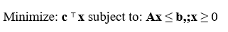
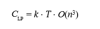
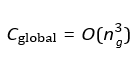
Where c is the cost vector, x is the vector of decision variables, A is the constraint matrix, and b is the constraint vector. The computational complexity of the simplex method depends on the structure of the problem. While it is polynomial for many practical cases, its worst-case complexity is exponential [26]. Modern interior-point methods have a theoretical complexity of:

Where n is the number of variables. As n and the number of constraints grow, the computational cost increases significantly. In real-time applications requiring frequent updates, if k updates occur per unit time, the total cost over a time horizon T is [27]:

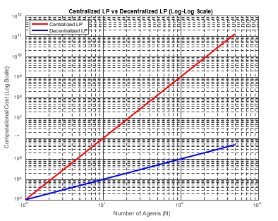
This scaling can become computationally prohibitive in large- scale, dynamic systems. Plugging these into a graph illustrates the point. Note linear programming is faster in low dimensional spaces by reducing recomputes, but practical wargaming contains an enormous number of variables [28].

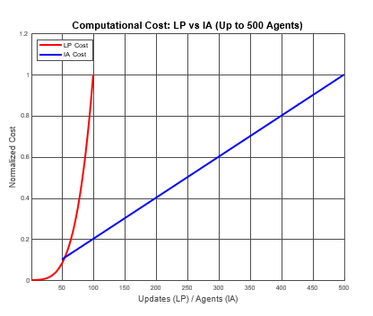
However, by using linear programming inside agents, the combinatorial explosion is reduced, due to the reduced dimensionality of the problem from the agents' perspective.

Agents and Linear Programming

Intelligent agents mitigate the combinatorial explosion problem by decentralizing decision-making. Each agent operates independently, responding to local conditions and data rather than attempting to solve the global problem [29]. This approach reduces computational requirements by focusing only on relevant subsets of the problem. Agents process live sensor data (or live simulated data) in real-time, adapting dynamically to changes such as weather shifts or enemy maneuvers. Decentralized systems naturally scale with the number of agents, as additional agents contribute to distributed computation rather than increasing global complexity. In missile salvos, intelligent agents can adjust their timing and trajectories autonomously, maintaining effectiveness even in unpredictable conditions.

Emergent behavior reveals optimizations that are often inaccessible to linear programming and other top-down approaches because it leverages local interactions and real-time data to produce system- wide dynamics. Linear programming models rely on explicitly defined constraints and objectives to compute globally optimal solutions for well-understood problems [30]. While effective for structured scenarios, these methods are limited by their static nature, assuming complete and accurate knowledge of the system at the time of computation [31]. This rigidity frequently excludes the adaptability required for dynamic environments.

In contrast, emergent systems use decentralized decision-making among agents, allowing the system to evolve in response to changing conditions. When on-the-fly sensor data is integratedinto these agents, the system becomes even more dynamic, enabling real-time adjustments that linear programming cannot accommodate. For instance, in a missile swarm engagement, agents equipped with real-time sensor inputs, such as target speed or trajectory changes, can adapt their behavior dynamically. These agents use updated local data to adjust their alignment, velocity, or target prioritization, collectively uncovering strategies such as multi-vector attacks or adaptive evasive maneuvers. These strategies emerge naturally from the interactions among agents and their continuous integration of new information.

Linear programming provides precision in solving predefined problems, such as optimizing an intercept trajectory based on current conditions, fuel constraints, or time-to-intercept requirements. However, these methods depend on static input data, making them less effective in environments where conditions shift rapidly. For example, if a target changes its trajectory unpredictably, a linear programming model would require re-computation of the entire solution. Emergent behavior, on the other hand, thrives in these scenarios because it does not rely on static constraints. Instead, the system dynamically updates its state as new sensor data flows to the agents, enabling continual adjustment to changing conditions.

The ability of emergent systems to use on-the-fly sensor data also enhances their scalability and robustness. In a distributed swarm of drones or missiles, each agent processes local sensor information independently, allowing the system to adapt without requiring centralized computation. This distributed nature means the system can handle disruptions, such as the loss of individual agents, without collapsing. In contrast, linear programming models often depend on centralized calculations, which can become computationally prohibitive for large-scale systems or fail under incomplete information. Emergent behavior also uncovers solutions that are not predefined in the system’s initial design [32-34]. For example, in a search-and-rescue scenario, drones equipped with real-time environmental sensors might discover optimized coverage patterns or cooperative resource allocation strategies as they interact with one another and the environment. These optimizations arise dynamically from the system’s response to real-world conditions, bypassing the need for explicit programming of all possible contingencies.

Integrating on-the-fly sensor data into intelligent agents enhances their ability to discover unique, context-sensitive solutions. While linear programming excels in deterministic environments with fixed constraints, it struggles to adapt to new data or unforeseen conditions. Emergent systems, powered by real-time inputs and decentralized decision-making, overcome this limitation by continuously exploring and adapting to their environment. This adaptability, combined with the ability to process and respond to live data, enables emergent systems to uncover optimizations and solutions that are invisible to traditional top-down methods. A hybrid model, where agents use linear programming for localized tasks while relying on emergent dynamics for global coordination, represents my preferred approach to tackling complex, dynamic problems. There is some evidence that this path will bear fruit [35].

Relative Computational Costs

The relative computational cost between linear programming (LP) and intelligent agents depends on the complexity and dynamic nature of the scenario. In highly complex scenarios, such as missile salvo coordination under changing conditions, these costs vary due to the inherent differences in how LP and intelligent agents process information and adapt to changes. Let’s explore this.

LP Computational Cost

Linear programming is inherently centralized and deterministic. The computational cost of solving an LP problem is primarily driven by:

• Number of Variables: The more variables involved (e.g., missile trajectories, timing), the larger the problem size.

• Number of Constraints: Each additional constraint increases the dimensionality of the feasible solution space.

• Solution Method: Algorithms like the simplex method or interior-point methods are efficient for small to medium-sized problems but can become computationally expensive as the problem scales.

• For highly complex scenarios involving hundreds of variables and constraints, the computational complexity grows polynomially or worse, depending on the algorithm used. Solving a single LP instance for a scenario with live sensor data or dynamic conditions can become infeasible in real-time if frequent recalculations are required. Recomputing the global solution every time new data arrives (e.g., updated target positions or environmental changes) significantly increases the cost, making LP less practical for real- time applications.

Computational Cost of Intelligent Agents

Intelligent agents rely on decentralized decision-making, where each agent processes a subset of the global information and interacts with other agents based on local rules. The computational cost for intelligent agents is distributed across the system and influenced by:

• Number of Agents: The cost scales with the number of agents but remains manageable because each agent performs localized computations.

• Complexity of Local Rules: Simple rules (e.g., align, avoid, and cohere in flocking) incur low computational costs, while more advanced behaviors, like predictive modeling or dynamic adaptation, require more resources per agent.

• Real-Time Sensor Integration: Agents processing live sensor data do so locally, reducing the overall system-wide computational load.

In highly dynamic scenarios, intelligent agents are computationally more efficient than LP because they do not require recalculating a centralized solution. Instead, agents adjust autonomously to changes, making them inherently scalable and better suited for real-time adaptation.

Key Differences in Computational Costs

Centralization vs. Decentralization

LP requires centralized computation, making it bottlenecked by the size of the problem. Intelligent agents distribute computations across the system, allowing them to scale linearly with the number of agents and respond dynamically to localized conditions.

Recalculation Costs

LP must recompute the entire solution whenever the scenario changes, such as when live sensor data updates constraints or objectives. This recalculation incurs significant computational costs in complex and dynamic environments. Intelligent agents continuously adapt without requiring a complete system-wide recalculation, making them computationally less demanding in dynamic scenarios. There is ongoing work regarding LP optimizations, but many of these focus on multi-staging, which is, coincidentally, what agents do; meaning that embedding LP in agents can address the performance issue while inheriting the other advantages agents offer. Other possible LP optimizations are compatible with IAs, such as probabilistic futures, transportation distance minimization, sensitivity analysis, and persistence [36- 41].

Scalability

For hundreds or thousands of variables, LP’s computational cost grows rapidly due to the increasing complexity of the feasible solution space. In contrast, intelligent agents handle the added complexity more effectively by distributing computations and focusing only on local interactions.

Real-Time Efficiency

LP struggles to meet the real-time demands of highly dynamic scenarios because solving large-scale problems under time constraints is computationally expensive. Intelligent agents, by operating autonomously and in parallel, are better equipped to handle real-time changes efficiently [42].

Intelligent Agents Complexity

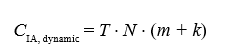
For intelligent agents, computational cost arises from local processing and interactions among agents. For a system with N agents, where each agent performs m computations per time step and interacts with k neighbors, the cost per time step is:

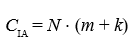
Here, m represents the cost of local computations, such as adjusting a trajectory, while k represents the interaction cost with neighboring agents. Unlike LP, intelligent agents do not require centralized recalculation. Over a time horizon T, the total cost is:

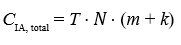
This linear scaling regarding N makes intelligent agents computationally more efficient for real-time operations in large- scale systems. Even in highly complex scenarios, agents have demonstrated computational speeds of up to 300 times faster than real time [43]. There is a communications cost (considered “edges”), so some effort needs to be expensed to keep bandwidth reasonable. For example, sending sensor data should be in the form of analysis results when possible, instead of raw pixels. We use shared memory mapping and when across different machines, sockets.

Comparative Scaling Models

In dynamic systems requiring frequent updates, the computational cost for LP and intelligent agents can be compared as follows. For LP, where recalculations are needed for every update:

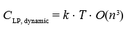
For intelligent agents processing updates locally and distributed across the system:

For large N or high-frequency updates, C_{IA, dynamic} scales more efficiently than C_{LP, dynamic}, particularly when n (the global variable set) grows faster than N (the agent count).

Mathematical Models for Decentralized Systems

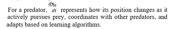
Emergent behaviors in intelligent agent systems can be modeled using dynamical systems and graph theory. The state xú i(t) of each agent evolves according to local rules and interactions:

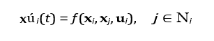
Where u_i represents sensor input, and N_i denotes the set of neighboring agents.

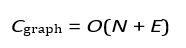
The global system behavior emerges from the network of agent interactions, represented by a graph with N nodes (agents) and E edges (interactions). The computational cost of managing these interactions scales as:

The cost difference between LP and intelligent agents is determined by their scaling properties. LP scales polynomially or worse with the number of variables and recalculations, making it less suitable for dynamic, largescale systems. Intelligent agents, with their distributed computations and linear scaling, are more efficient for handling real-time adaptability. The equations demonstrate why intelligent agents are preferred in scenarios involving frequent updates, decentralized operations, and emergent behaviors.

Large Scale Hybrids

By using linear programming (LP) within agents, the dimensionality of the problem is localized to each agent’s perspective, significantly reducing the computational overhead associated with the global problem. This approach leverages the decentralized structure of intelligent agents while still benefiting from the optimization capabilities of LP for specific subproblems.

Localization of Problem Dimensionality

In a global optimization framework, the entire problem, including all variables, constraints, and interactions, must be solved simultaneously. As discussed, this typically leads to a combinatorial explosion as the number of variables and constraints increases. In contrast, when LP is embedded within individual agents, each agent focuses only on its immediate environment and tasks. This localization reduces the problem’s dimensionality because:

• The agent considers only variables relevant to its actions (e.g., trajectory adjustments, local resource allocation).

• Constraints are limited to those directly affecting the agent, such as its speed, turn radius, or proximity to other agents.

For example, in a missile swarm scenario, each missile agent might use LP to optimize its trajectory and timing to avoid collisions while maintaining alignment with broader mission goals. The global problem of coordinating the entire swarm is thus broken down into manageable local optimizations. The global problem then is solved via asynchronous swarming, producing what is typically called emergent intelligence [44].

Reduction in Computational Overhead

The localized use of LP significantly reduces computational overhead compared to solving a centralized LP problem. For an agent with na variables and ca constraints, the computational cost of solving its LP is proportional to:

Where n_a and c_a are typically much smaller than the total number 106 of variables and constraints in the global system. In a system with N agents, each performing independent LP computations, the total cost scales as:

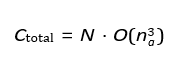
This scaling is far more efficient than solving a centralized LP with n_g variables, where:

and n_g can be orders of magnitude larger than n_a ⋅ N due to interdependencies among all agents in the centralized model.

Improved Scalability

By distributing LP computations among agents, the system becomes more scalable as the number of agents increases. Each agent independently processes its localized problem, and the addition of new agents introduces additional computational capacity rather than exponentially increasing the problem’s complexity. This scalability is particularly advantageous in large- scale, dynamic environments, such as coordinating hundreds of missiles in real-time under changing conditions.

Dynamic Adaptation and Real-Time Optimization

Embedding LP within agents also enhances the system’s ability to adapt dynamically to changing conditions. Each agent can re-solve its localized LP problem in real time as new sensor data becomes available or as environmental variables change. For example:

• A missile agent might adjust its trajectory based on updated enemy movements or environmental factors like wind speed.

• A drone swarm agent might optimize its resource allocation to prioritize specific tasks in response to changing mission objectives.

This real-time adaptability is challenging in a centralized LP framework, where the entire problem must be recalculated whenever any variable changes. A comparison is shown below, where LP is embedded into agents, which still yields non-linear computational growth, but in a more controlled fashion due to dimensionality reductions.

Maintaining Global Objectives Through Coordination

While agents optimize locally, they can still align with global objectives through limited communication and coordination. By sharing key parameters or constraints with neighboring agents, the system ensures that local LP solutions contribute to the overall mission’s success.

For example:

• Neighboring missiles might exchange data on timing and trajectory to avoid interference.

• A swarm of drones might use local LP to optimize energy usage while collectively ensuring coverage of a target area.

Local Optimization for Missile Systems Using Linear Programming

The opportunities for incorporating linear programming into missile systems are essentially the same as in global optimization frameworks. However, by embedding LP within individual missile agents, optimization becomes localized, focusing on the specific dynamics and tasks of each missile. This localized approach enables dynamic adaptability and reduces computation, while maintaining alignment with broader mission objectives.

Intelligent Agents

All missile intercept dynamics components, including real- time adjustments, guidance laws, and handling of unpredictable targets, can be encoded into intelligent agents. These agents make autonomous decisions based on input data, optimized for specific objectives, and use simulated or real sensor input. Proportional navigation and its augmentations naturally map to the functions of intelligent agents.

Proportional navigation

The core aspects of the guidance system, not including swarming social behavior, can be summarized as follows:

The agent must continuously process real-time inputs, such as the target’s position, velocity, and acceleration. This information can be obtained through sensor fusion, where radar, infrared, or other tracking systems provide the agent with an updated state of the target. The relative position r(t) and line-of-sight (LOS) angle λ can be calculated as inputs to the guidance system. LOS  rate λ and closing velocity V_c must be dynamically computed, forming the basis for trajectory adjustments. The agent must implement the proportional navigation (PN) guidance law. Using the relationship ac = N ⋅ V_c ⋅ λ^., the agent determines the lateral acceleration required to intercept the target. This computation can be encapsulated in a decision-making module that considers both current dynamics and the physical capabilities of the interceptor, such as maximum acceleration or turn radius. The agent should adapt to unpredictable changes in the target’s motion. This can be achieved through predictive modeling, such as Kalman filters, which estimate the target’s future trajectory based on noisy or incomplete data. For highly dynamic targets, the agent can employ augmented proportional navigation, where additional terms like a_T (target acceleration) are incorporated into the guidance law.

The agent must manage the interceptor’s constraints, such as range, speed, and maneuverability. For example, the agent may simulate future states of the target and interceptor to determine whether the intercept is feasible within the operational range and time constraints. If infeasible, the agent may recommend course adjustments or resource reallocation. Requiring movements outside its stability envelope will most likely destroy the vehicle.

Graph-Based Pairing

Agents may maintain distant pairings and interleave local non- paired, but friendly agents. This provides for better Intelligence, Surveillance, and Reconnaissance (ISR), due to increased baseline distances. To accomplish this involves leveraging frameworks like state machines, optimization algorithms, and machine learning models. Each aspect of the intercept dynamics can be represented as modular behaviors, allowing agents to operate autonomously while adhering to the physical and operational constraints of missile defense systems. The flexibility and adaptability of intelligent agents make them well-suited for complex and dynamic missile intercept tasks

Integrated Machine Learning

The agent’s behavior can be enhanced with machine learning to optimize performance over time. By training on simulated engagements, the agent can learn to adjust parameters like the navigation constant N or improve its response to highly agiletargets. This learning-based adaptation enables the system to generalize across a wider range of scenarios.

Network Centric

Intelligent agents can integrate higher-level objectives beyond single intercepts. For example, they can coordinate with other agents in a network, assigning interceptors to targets based on threat prioritization, available resources, or mission constraints. This multiagent coordination ensures optimal resource utilization in complex engagement scenarios. This ability is necessary for salvo sequencing and critical path optimization.

Neuroevolution

Neuroevolution with adaptive neural architectures enables dronesto adapt their neural architectures dynamically rather than relyingon fixed structure. Unlike traditional AI models, which operate with predefined structures, these drones develop optimal synaptic connections in real-time, adjusting to environmental changes and mission requirements. This adaptability is achieved through techniques such as Neuroevolution of Augmenting Topologies (NEAT), where the system evolves increasingly complex neural structures without manual intervention. Although the terminology surrounds genomes, the implementation is effective a set of connection lookup tables, plus flexibility in activation functions and weights. There are two key tables; genes and synapse lookup.

Node ID	Type	Activation Function	Bias
1	Input	Linear	0.0
2	Input	Linear	0.0
3	Hidden	Sigmoid	-0.1
4	Hidden	Tanh	0.3
5	Output	Softmax	0.0

Gene Table

Innovation ID	From Node	To Node	Weight	Enabled	Historical Marker
1	1	3	0.75	Yes	1001
2	2	3	-0.42	Yes	1002
3	3	5	1.21	Yes	1003
4	2	4	0.34	Yes	1004
5	4	5	-0.67	Yes	1005
6	1	5	0.88	No	1006 (Disabled)

Synapse Lookup

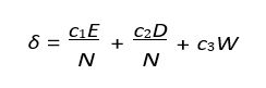
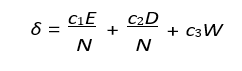
Upon learning, we apply “mutations” to initiate change. For example, for adjusting weights:

Where:

– E = Excess genes.

– D = Disjoint genes.

– W = Average weight difference.

– c₁, c₂, c₃ = Speciation coefficients.

– N = Normalization factor. For adding new connections:

For adding new connections:

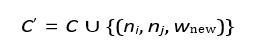
Where w_new is a random weight.

For splitting existing connections:

C′ = (C − {(n_i, n_j, wold)}) ∪ {(n_i, nnew, 1), (nnew, n_j , wold)}

Networks are clustered into species based on similarity as:

Where:

– E = Excess genes.

– D = Disjoint genes.

– W = Average weight difference.

– c₁, c₂, c₃ = Speciation coefficients

. – N = Normalization factor.

We may also have crossover (recombination), where connection ta- bles and historical tables are mixed, or some random connections are enables as a form of mutation. Adjusting the hyper parameters surrounding these can have a dramatic impact, and so modification based on reinforcement typically works best. A key advantage to neuroevolution is resilience to hardware failures. If a sensor fails, drones can adjust to use alternative inputs, maintaining effective- ness. This adaptability extends to real-time learning, where drones optimize flight control through reinforcement learning. This makes them useful for unpredictable threats or rapidly changing battlefield conditions.

Synaptic plasticity enables drones to learn and restructure their decision-making processes over time. Unlike rigid control systems, drones with neural plasticity introduce emergent intelligence, allowing them to adapt fluidly to threats and optimize approaches. This technology is particularly advantageous in unmanned autonomous combat vehicles (UAVs), that must adapt to enemy countermeasures, and surveillance and reconnaissance drones that learn to refine tracking behaviors based on terrain and environmental conditions.

Neuroevolution enables drones to adapt to mission constraints, optimizing coordination without centralized control. Formations can autonomously shift based on enemy presence, objectives, and communication. Selfmodifying neural networks enhance drone fleet efficiency and survivability, making them adaptable to military and non-military applications. There are challenges, however. One of the primary challenges in neuroevolution is its computational cost related to slow convergence. Unlike traditional gradient-based methods such as backpropagation, neuroevolution requires evaluating a population of networks across multiple generations, which can be expensive in terms of both time and resources. As networks grow in size and complexity, the number of evaluations required increases exponentially. Furthermore, unlike gradient-based learning, where network size is predetermined, neuroevolution dynamically grows network topologies. This can lead to excessive complexity, known as bloat, where the networks become larger than necessary without improving performance. Neuroevolution operates at the macro level, modifying an entire network instead of adjusting individual weights like backpropagation. This leads to difficulty in assigning credit to specific mutations or structural changes. Finally, unlikedeep learning models that can leverage pre-trained features, neuroevolved networks are taskspecific, making it difficult to transfer knowledge to new domains. All that being said, this is one area where dramatic progress can be made with minimal coding.

Heterogeneous Drugs

Unmanned aerial systems (UASs) have emerged as a key asset in ISR operations and electronic warfare, supporting both strike mission planning and missile defense. We evaluate their role within the ISR-Strike cycle and assess their implications for adversary defensive planning. We consider them in the production of cost maps and afterstrike battle damage analysis.

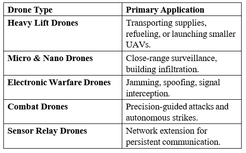
Heterogeneous drone systems leverage multiple specialized UAV types rather than relying on a homogeneous fleet. Each drone class is designed for a specific function, leading to a more robust and efficient deployment strategy. Heavy lift drones carry supplies or deploy smaller UAVs, while micro and nano drones operate in confined spaces or execute close-range surveillance. Electronic warfare drones are responsible for jamming, spoofing, and signal interception, whereas combat drones are equipped with precision- guided weapons. Sensor relay drones extend the operational network, ensuring uninterrupted data flow even in communication- denied environments.

The effectiveness of a heterogeneous drone fleet depends on task allocation algorithms that dynamically assign roles based on mission objectives and real-time constraints. Multi-agent coordination ensures that each drone performs optimally within the larger system, adjusting its function as needed. This approach is particularly useful in contested environments, where attrition is expected, and redundancy must be built into the system. If a combat drone is lost, others can take over its function, or support drones may adapt to fill the gap.

Heterogeneous drone systems offer significant energy efficiency advantages. Specialized units handle specific tasks, reducing overall energy consumption. Smaller drones perform low-power reconnaissance, while larger units reserve power for strikes. Dynamic role reassignment enhances fault tolerance, making the system resilient to enemy counter measures.

Heterogeneous drone systems are widely used in ISR missions, where diverse sensor capabilities are deployed across a battlefield. Dynamic targeting, where AI determines which drones engage threats, is another key application. In multi-domain operations, these drones coordinate across air, sea, and land for mission success in complex environments.

Bio Hybrid Drones

We have been doing research on observing birds in real-time during flight, which may be thought of as a collection of flying sensors. By modeling them as a collection of oblique cameras, we can observe not only objects competing for airspace or threats, but we can also begin to understand athmospherics. Let’s discuss in more detail.

Bio-hybrid drones incorporate biomimetic flight inspired by birds, bats, and insects, allowing for increased maneuverability, energy efficiency, and stealth. By studying avian flight patterns, these drones replicate complex aerodynamic behaviors that provide significant advantages over traditional UAV designs. Morphing wing structures allow for real-time adjustments in shape, angle, and stiffness, optimizing aerodynamics in response to turbulence and wind conditions.

One of the most effective techniques derived from birds is dynamic soaring, where drones exploit natural air currents to extend endurance without excessive power consumption. Similarly, perching behaviors enable drones to land on structures, reducing energy usage while conducting passive surveillance. By mimicking flocking behaviors, bio-hybrid drones gain additional advantages in energy conservation and deception, blending into natural bird formations to avoid detection. Different bird species provide inspiration for distinct drone functionalities. Falcons influence high-speed strike UAVs designed for rapid engagement, while albatross-based drones specialize in long-range endurance missions. Peregrine-inspired drones optimize urban navigation with agile flight paths, while owl-like designs emphasize stealth operations through noise reduction.

Bio-hybrid drones provide unique advantages in both covert operations and endurance-based missions. Their ability to integrate into natural flight patterns makes them particularly effective for ISR in contested environments where traditional UAVs would be easily detected. By reducing energy dependency and enhancing aerodynamic performance, these drones are well suited for urban reconnaissance, battlefield surveillance, and long-duration operations where power conservation is critical.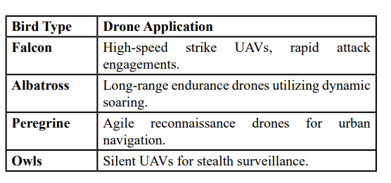

Lotka Volterra

Alfred James Lotka (1880–1949) was an American theoretical biologist, mathematician and practical joker. He is best known for his pioneering work in population dynamics, energetics and applying predator-prey mathematics to the insurance industry (much to the amusement of his co-workers at Metropolitan Life Insurance).

Vito Volterra (1860–1940) was an Italian mathematician and physicist but an academic outsider. He is best known for theoretical ecology, but made significant contributions to functional analysis, partial differential equations, and integral equations. He was deeply fascinated by fish populations, which led to his development of the predator-prey equations. Furthermore, he would sometimes humorously refer to fishermen as “accidental ecologists” because their records of catches indirectly provided data for his models.

Nicolas Rashevsky (1899-1972) was a Ukrainian-American theoretical biologist and a pioneer in mathematical biology. He studied in Russia and immigrated to the US to escape the Russian Revolution. Rashevsky established the first journal dedicated to mathematical biology, The Bulletin of Mathematical Biophysics, and spent his career at the University of Chicago. Rashevsky combined the works of Lotka and Volterra. Like Lotka and Volterra, many biologists of Rashevsky’s time were skeptical of applying abstract mathematics to biology, seeing it as overly reductionist or disconnected from empirical observation. Nonetheless, his vision of a mathematically rigorous approach to biology proved influential and gave us the foundations of intelligent agents. These three individuals collectively revealed the Predator-Prey mechanism in use today. Of course, their work was based on even earlier works, but these three individuals molded what we see today as a biological principle [45].

Predator-Prey

The Lotka–Volterra equations can be adapted for missile-to- missile intercept simulations by treating incoming threat missiles as the prey and interceptors as the predators [46,47]. The equations are written as:

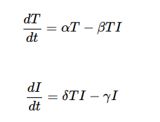
Where T (t) is the number of threat missiles, and I(t) is the number of interceptors. The parameter α represents the rate of new incoming threats, β reflects the engagement efficiency of interceptors,, δ  represents the rate at which threats convert into successful defensive actions (e.g., launches of additional interceptors), and γ accounts for the depletion of interceptors over time due to resource or operational constraints.

The term αT models the growth of the threat missile population, reflecting the arrival of additional salvos or missiles over time. The interaction term − βTI captures the rate at which interceptors neutralize threats. For interceptors, δ TI represents the deployment or activation of more interceptors in response to the incoming threat, while −γI accounts for natural depletion, such as resource exhaustion or missed interceptions.

Mathematical Models for Predator-Prey

The Lotka-Volterra model mathematically represents predator-prey dynamics through a system of differential equations that describe changes in predator (P) and prey (R) populations over time. The prey population grows at a rate proportional to αP butdecreases due to predation at a rate βPR, where β represents the predation rate coefficient. Conversely, the predator population increases based on successful predation, captured by δPR, with δ representing the efficiency of converting prey into predatoroffspring, while naturally declining at a mortality rate.

This model establishes a foundational framework for understanding cyclic oscillations in predator-prey populations; however, it simplifies real-world dynamics by omitting critical factors suchas spatial distribution, adaptive behaviors like learning, and social cooperation, which influence ecological stability and complexity in natural systems.

This is expressed as:

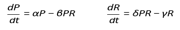
Where:P = Predator population

R = Prey population

α = Prey growth rate

β = Predation rate coefficient

δ = Predator reproduction efficiency

γ = Predator mortality rate

This model provides a baseline but lacks spatial movement, learning, and cooperative behaviors.

Pursuit-Evasion Equations (Optimal Predator Pathing)

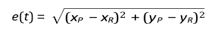
The pursuit-evasion equations model the dynamics of predator- prey interactions through optimal control theory, where both predator and prey adjust their movement strategies to achieve opposing objectives. The predator’s position (x_P, y_P) and the prey’s position (x_R, y_R) evolve based on their respective speeds (v_P, v_R) and movement angles (θ_P, θ_R), described by differential equations that account for their directional velocities. The predator aims to minimize the Euclidean distance to the prey, optimizing its path to intercept efficiently, while the prey seeks to maximize this distance to enhance its chances of escape. This framework extends beyond biological contexts, such as in drone swarm evasion scenarios where stealth drones (prey) minimize their detectability usingwhere stealth drones (prey) minimize their detectability using
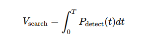
Conversely, interceptors (predators) focus on minimizing tracking error, e (t), to improve interception accuracy. In antisubmarine warfare (ASW), similar principles apply, with evasion probability increasing exponentially with distance from detection sources, modeled byP _evade = e^−αd, where α represents the attenuation factor of the medium. Optimal search patterns in ASW are quantified through the integration of detection probability over time, providing strategic insights into maximizing detection efficiency during operations.

Optimal control theory may be expressed as:

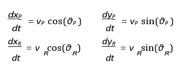
Where:

(x_P , y_P) = Predator coordinates

(x_R , y_R) = Prey coordinates

v_P ,v_R = Speeds of predator and prey

θ_P , θ_R = Movement angles

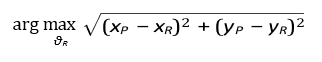
Path Optimization

  – The predator minimizes the Euclidean distance:

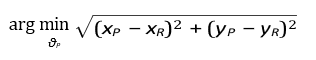
  – While the prey maximizes escape distance: 

A practical example of this is drone swarm evasion, where prey (stealth drones) maximize low-observability:

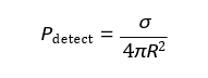
Where:

σ = Radar cross-section (RCS)

R = Distance to radar

 –Predators (interceptors) minimize tracking error:

A variate being ASW, with a sonar evasion probability of:

Where:

d = Distance from detection source

α = Medium-dependent attenuation factor

– Optimal search patterns for ASW:

Pack Coordination (Multi-Agent Predator Strategies)

Formation control for pack hunting models how predators coordinate their movements using graph-based formations, where each predator adjusts its position based on the relative positions of its neighbors. This coordination is described by the force equation F_i = ∑_j∈Ni k_ij (x_j − x_i), where x_i represents the position of the predator i, Ni is the set of neighboring predators, and k_ij denotes the strength of coordination with the predator j. This interaction ensures cohesive group movement, allowing predators to maintain effective hunting formations. In the encirclement model, predators strategically position themselves to form a convex hull around the prey, effectively trapping it within a defined hunting zone. This is 

 

where r _encirclement defines the radius within which the prey is contained, and N_P represents the number of predators involved. This approach facilitates dynamic encirclement strategies, enhancing the efficiency of coordinated hunting in both biological systems and applications such as autonomous drone swarms executing cooperative interception tasks.

Formation Control for Pack Hunting

Predators coordinate positions based on graph-based formations:

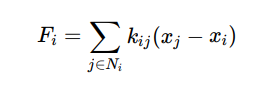
Where: x_i = Position of predator i

k_ij = Coordination strength with neighboring predator j

Ni = Set of neighboring predators

Encirclement Model

Predators form a convex hull around prey:

 

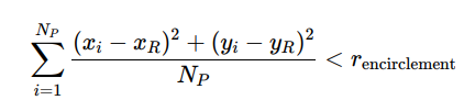
Where r_encirclement defines the hunting zone.

Prey Evasion

Randomized Escape Paths

Prey use stochastic movement to avoid predictable tracking:

Where:

σ = Standard deviation controlling randomness

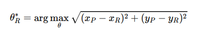
Optimal Escape Angle

Prey selects an angle maximizing distance to predator:

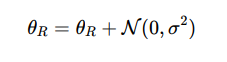
AI-Based Learning (Reinforcement Learning in Predator- Prey)

Prey evasion strategies often incorporate stochastic movement to reduce predictability and improve survival against tracking predators. This behavior is modeled by introducing Gaussian noise to the prey’s escape angle, represented as θ_R = θ_R + N (0, σ²), where N (0, σ²) denotes a normal distribution with zero mean and variance σ², and σ controls the degree of randomness in the movement. By adding this stochastic component, prey can avoid following easily anticipated paths, making it more challenging for predators to predict their trajectory. Despite this randomness, prey still aim to optimize their escape by selecting an angle that

of random perturbations with distance-maximizing strategies enhances evasion effectiveness, balancing unpredictability withgoal-oriented movement to improve survival odds in both natural ecosystems and engineered systems such as autonomous vehicles evading hostile tracking.

Predator Reward Function (Hunting Efficiency)

Predators maximize hunting success with a reward function:

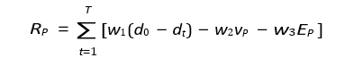
Where:

d₀, d_t = Initial and current predator-prey distances

v_P = Speed penalty

E_P = Energy cost for movement

w₁, w₂, w₃ = Weight coefficients

Prey Reward Function (Survival Maximization)

Prey maximize escape probability:

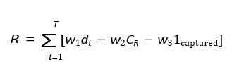
Where:

C_R = Energy cost of movement

1_captured = Binary indicator (1 if captured, 0 otherwise)

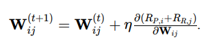
Multi-Agent Evolutionary Adaptation

Multi-agent evolutionary adaptation models the co-evolution of predators and prey through genetic algorithms, where both populations iteratively adjust their behaviors to improve survival

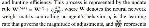
the gradient of the reward function R regarding the weights. Thereward function differs for predators and prey, reflecting objectives such as successful capture or effective evasion. Over successive generations, mutation, and crossover operators introduce variations in behavioral strategies, enabling the emergence of complex,adaptive responses. This evolutionary framework simulates the dynamic arms race observed in natural ecosystems and is applicable to artificial intelligence systems, where autonomous agents learn to optimize strategies through iterative competition and adaptation.

Predators and prey co-evolve using genetic algorithms:

Where:

W = Neural network weight matrix

η = Learning rate

R = Reward function (predator or prey)

Mutation and crossover operators modify behaviors over generations.

Tying it Together

These equations extend traditional flocking to adaptive predator- prey behaviors through:

1. Optimal control & pursuit-evasion mechanics.

2. Multi-agent cooperation & coordination.

3. Reinforcement learning & evolutionary AI.

4. Real-world tactical applications in drones, ASW, and EW.

To describe the behavior of a single agent and then generalize it to multiple agents, we formulate an individual-based model that captures dynamics related to population interaction, movement, learning, and detection. The dynamics for a single predator-prey pair are defined as follows:

Individual-Based Dynamics

For a single predator i and prey j, the system can be expressed as:

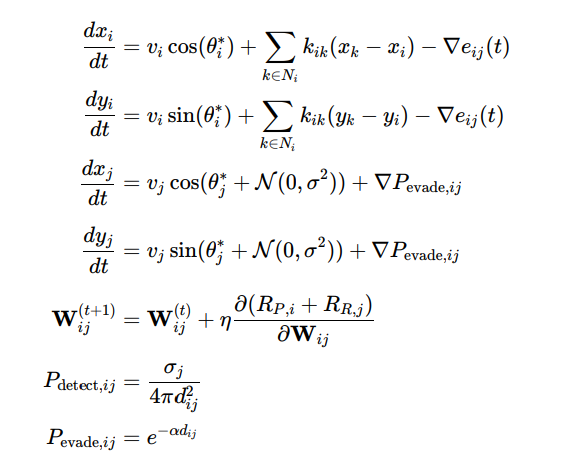
Where:

–  (x_i,y_i) and (x_j,y_j) are the coordinates of predator i and prey j.

–  v_i, v_j are their respective speeds.

–  θ_i * and θ_j * are optimized pursuit and evasion angles

–  N_i is the set of neighboring predators for coordination, with kik representing coordination strength.

–  e_ij (t) is the tracking error between predator i and prey j

–  P_{detect, ij} is the detection probability depending on radar cross section σj and distance d_ij.

– • P_evade,ij is the evasion probability, decreasing with distance dij and attenuation factor α.

– W_ij is the neural network weight matrix controlling adaptive behaviors through reinforcement learning.

Generalizing to Multiple Agents

To extend this to multiple predators (N_P) and prey (N_R), we sum over all agents:

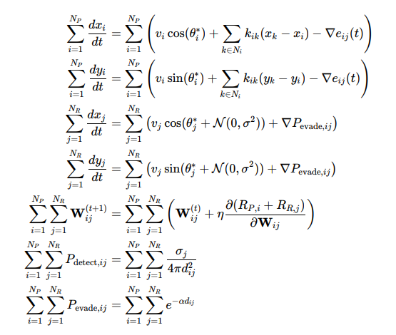
Transition from Multi-Equation System to Unified Agent- Based Model

The transformation from the set of equations representing separate dynamics for predators and prey to a unified agent-based model involves several key steps. The goal is to generalize the behavior of all agents (both predators and prey) under a single, compact notation.

Step 1: Identifying Common Dynamics

In the original system:

– Predator Dynamics (Position Updates): x and y components evolve based on speed, direction, coordination with neighbors, and error minimization.

Example terms: v_i cos(θ^*_i),

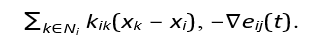
– Prey Dynamics (Position Updates): Similar to predators, butwith stochastic noise to model evasion: N (0, σ²) and ∇P _evade,ij.

–Learning Dynamics (Weight Updates): Neural weight updates

Detection and Evasion Probabilities: P detect,ij and P evade,ij depending on distances and environmental factors.

Step 2: Generalizing Variables for All Agents

Instead of handling predators (i) and prey ( j ) separately, we define:

– General agent index: a = 1, 2,...,N, where N = N_P +N_R (total number of agents).

– Position vector: x_a = (x_a ,y_a) for each agent.

Velocity: v_a with direction θ_a (optimal for pursuit or evasion).

Coordination term: ∑ b_∈Na k_ab (x_b −x_a) applies to all agents,generalizing neighbor influence

Adaptive behavior: ∇R_a represents the reward gradient applicable for both predators (capture success) and prey (evasion success).

Stochastic behavior:N (0, σ² ) captures randomnes sprimarily affecting prey but included for generalization.

Step 3: Combining into a Single Equation

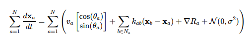
Merging all components into one expression for position updates:

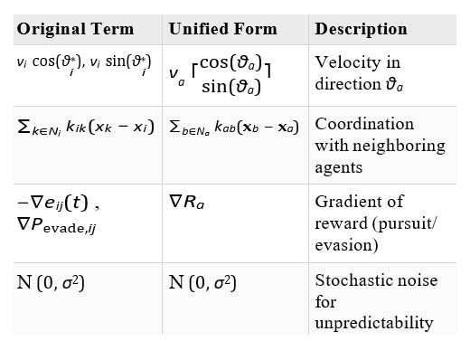
step 4;Mapping Terms from Original to Unified Form

Simplifications

–• Abstraction of Agent Roles: By replacing predator/prey indices (i, j) with a universal agent index (a), we eliminate the need to write separate equations for each role.

–• Unified State Update: All agents update their positions according to the same rule, with role-specific behavior embedded in parameters like R_a (reward function) and θ_a (optimal direction).

–• Compact Notation: This format simplifies representation, making it easier to scale to large multi-agent systems, such as drone swarms or missile interception networks.

In essence, we’ve transitioned from a role-specific, multi-equation system to a generalized agent-based framework that captures the dynamics of all entities within a single cohesive expression, ij ij ∂Wij simplifying our life.

This multi-agent formulation captures the full dynamics of predator-prey interactions, including pursuit-evasion mechanics, coordination in packs, stochastic evasion behaviors, and adaptive learning through reinforcement mechanisms.

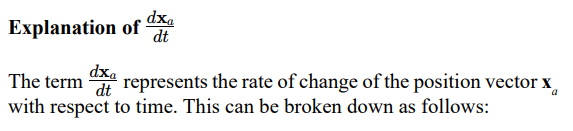
x_a: This is the position vector of agent a, defined as x_a = (x_a, y_a)in a two-dimensional space.

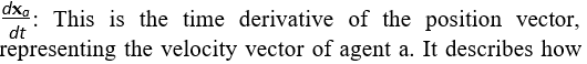
the position of the agent changes over time in both the x and y directions. In component form:

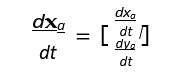
This vector gives the instantaneous velocity of agent a in both spatial dimensions.

Breakdown of the Right-Hand Side

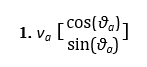
– This term represents the self-propelled motion of agent a, where va is the speed and θa is the movement direction.

– It defines the agent’s movement based on its current heading.

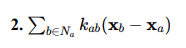
– This models the influence of neighboring agents.

– The term (x_b − x_a) is the vector pointing from agent a to its neighbor b, and k_ab is the strength of this influence. – It accounts for behaviors like formation control or flocking.

3. ∇Ra – This is the gradient of the reward function, representing the adaptive behavior of the agent (e.g., moving toward a target for a predator or maximizing escape routes for prey).

– It reflects how the agent adjusts its behavior to optimize its objective, such as maximizing capture probability or evasion success

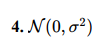
– This term introduces stochastic noise to the movement, typically modeled as Gaussian noise with mean 0 and variance σ^2.

– It adds randomness, simulating unpredictable behaviors such as evasive maneuvers in prey.

Physical Interpretation

For prey, it represents how its position changes as it evades predators, responds to the environment, and introduces randomness to avoid predictability.

of self-propulsion, interaction with other agents, adaptive learning, and stochastic perturbations.

Alignment with Mission Objectives

Although each missile optimizes locally, their solutions remain aligned with overall mission objectives through limited com- munication and coordination. For example, missiles targeting a high-value asset might exchange timing or trajectory parameters to ensure synchronized salvos or coordinated approaches from dif- ferent angles. This balance between local optimization and global alignment is important for successful multi-missile engagements.

Incorporation of Missile Dynamics

To accurately simulate missile-to-missile engagements, additional missile dynamics, alluded to in the proportional navigation discussion, must be included to account for real-world operational limitations.

Turn Radius

The minimum turn radius, r_min, depends on the missile’s speed v and maneuverability, often modeled as:

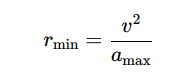
Where a_max is the maximum allowable lateral acceleration. This affects the intercept probability and engagement windows, as missiles may be unable to adjust trajectory quickly enough to pursue agile threats.

Speed

Missile speed, v, directly impacts the engagement timeline and the probability of successful interception. Faster interceptors can close the distance to threats more rapidly, increasing β, the engagement efficiency. However, high-speed interceptors may have limited maneuverability, reducing their effectiveness against slower but more agile threats.

Flight Profiles

Missiles follow specific flight profiles (e.g., ballistic, cruise, or direct pursuit), which influence their engagement capabilities. Profiles determine the missile’s trajectory, including altitude, path curvature, and terminal-phase maneuverability. For example:

–  Direct pursuit leads to faster engagements, but may result in higher fuel consumption and earlier depletion of resources.

– Cruise profiles maximize range but may delay the engagement timeline, affecting β.

Range

Each missile has a finite operational range, R_max. Engagements can only occur if the target is within this range. This introduces a spatial constraint, limiting T(t) and I (t) interactions to scenarios where threats and interceptors overlap within their respective ranges. The effective engagement rate is modified to:

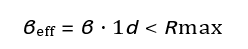
Where 1 d < Rmax is an indicator function that equals 1 if the distance d between missile and target is within the interceptor’s range, and 0 otherwise.

Modified Model for Dynamics

The interaction term −βTI can be expanded to include these dynamics:

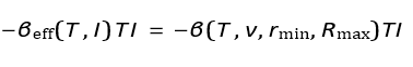
This ensures that interception rates depend on physical limitations such as speed, maneuverability, and range.

Practical Implications

The integration of missile dynamics into the model provides a more realistic representation of missile-tomissile engagements. Threats with high agility and evasive maneuvers reduce effective engagement rates, β, requiring interceptors to have sufficient speed and maneuverability. Engagements must also consider range limitations, as interceptors cannot engage targets beyond their operational radius. Additionally, engagement timelines are affected by the time required for interceptors to adjust trajectory, particularly against threats with advanced profiles or decoys.

Review of Proportional Navigation

The normal closed-loop solution for missile intercept using Proportional Navigation (PN) involves the following mathematical framework:

The lateral acceleration command is given by:

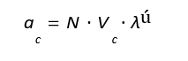
Where a_c is the lateral acceleration, N is the navigation constant, V is the closing velocity, and λ is the rate of change of the line-of- sight (LOS) angle.

Key Variables and Dynamics

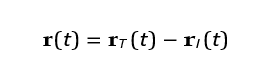
The relative position vector between the interceptor and the target is:

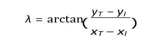
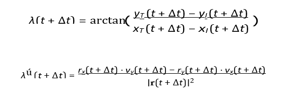
The LOS angle λ is defined as:

The LOS rate λ is calculated as:

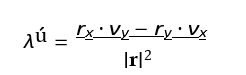
Where r_x = x_T − x_I and r_y = y_T − y_I are the relative position components, and v_x = v_T,x − _vI,x and v_y = v_T,y − v_I,y are the relative velocity components.

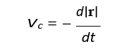
The closing velocity is:

The interceptor applies an acceleration proportional to the LOS rate:

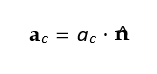
Where n^ is the direction perpendicular to the LOS vector.

Position and Velocity

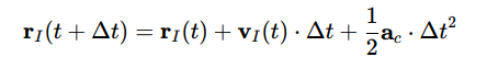
The position of the interceptor and target is updated iteratively. For the interceptor:

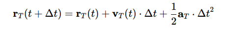
For the target:

LOS Rate

After updating the positions, the LOS angle and its rate are recalculated as:

Trajectory Convergence

The trajectory converges when the relative distance |r(t)| approaches zero. The closing velocity V_c ensures this convergence dynamically as the interceptor adjusts its path. Numerical integration methods, such as Euler or Runge-Kutta, can be used to solve these equations iteratively over time steps Δt, updating the positions and velocities of the interceptor and target until |r| <,€ where € is a small threshold for successful intercept.

This solution provides for on-the-fly changes in opposing missile dynamics by continuously adapting the interceptor’s trajectory based on real-time feedback. This capability is built into the system, as it relies on continuous updates to the line-of-sight (LOS) angle λ and its rate of change λ . Any changes in the opposing missile’s dynamics, such as speed, acceleration, or direction, arereflected in the relative position r(t) = r_T (t) − r_I (t) and the LOS rate

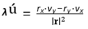
where r_x and r_y are relative position components, and v_x and v_y are relative velocity components.

The acceleration command ac = N ⋅ Vc ⋅ λú , recalculated dynamically, ensures the interceptor’s trajectory is continuously adjusted to account for the target’s new motion. The feedback loop ensures that deviations in the target’s path are addressed in real- time, dynamically modifying the lateral acceleration ac to maintain the intercept course. For example, if the opposing missile executes a sharp turn, the increased LOS rate λ prompts the interceptor to apply a greater lateral acceleration to stay on course.

The system’s effectiveness in handling dynamic targets depends on several factors, including the navigation constant N, the interceptor’s physical maneuverability, and the closing velocity V_c. A higher navigation constant improves sensitivity to LOS changes, but may result in overcorrection. The interceptor’s maximum lateral acceleration and turn radius determine its ability to respond to agile targets, while the closing velocity dictates the available response time.

For highly unpredictable targets, PN may be augmented with additional methods. Augmented Proportional Navigation includes

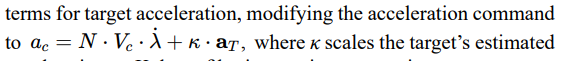
acceleration a_T. Kalman filtering can integrate noisy measurements to provide smoothed and predictive estimates of the target’s motion. Optimal control laws can further refine the guidance by minimizing a cost function that accounts for time-to-intercept, energy efficiency, and accuracy.

Proportional Navigation becomes important in understanding the destabilization of missiles during aggressive maneuvers or evasion. This is required when evading counter offensive weapons or when attacking highly agile or unpredictable targets. In theory, the onboard computers could prevent movements that destabilize the craft, but there are atmospheric factors the missile does not monitor. Since the simulator has knowledge of these conditions, and the missile does not, it can predict missile failure due to incorrect flight computer assumptions. Assuming the missile survives its encounter, proportional navigation also can determine the higher fuel consumption requirements of such maneuvers, and if the missile is then still within range of its target after such encounters.

Population

Population correlates to missiles running out of fuel, new missiles being launched, or missiles being destroyed at interception. The prey (enemy missile) population dynamics are modeled by the equation:

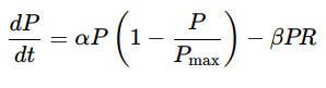
Where P (t) represents the number of prey at time t, α is the prey’s growth rate, and P_max is the maximum allowable prey population.

The predation term, −βPR, reduces the prey population based on the interaction between prey P and predators R, with β reflecting the efficiency of predation.

The predator population dynamics are governed by the equation

at time t. The term δPR models predator population growth proportional to the prey they consume, with δ representing the efficiency of converting prey into predator growth. The term −γR models the natural energy depletion of predators over time, where γ is the depletion rate. In the code, predators are removed when their energy reaches zero (run out of fuel), corresponding to −γR dominating over δPR.

The spatial dynamics of prey are described by r_P = r_P + v_P ⋅ d_t and v_P = v_P + €_P , where r_P is the prey’s position, v_P is its velocity, dt is the time step, and €_P represents random perturbations to mimic stochastic evasive movement. Prey reproduction follows

approaches P_max.

The predators’ spatial dynamics involve targeted movement toward prey. The position update is given by r = r_R + v_R ⋅ dt, and velocity updates are conditional on prey proximity. If prey is within range:

Where k scales the pursuit intensity. If no prey is nearby, velocity updates involve search patterns or random perturbations (loiter or scan). In the case of loiter, we can use:

The energy dynamics of predators are modeled by

Where E_R is the energy level of the predator, c is the energy depletion rate, g is the energy gained by consuming prey, and 1d < d_capture is an indicator function equal to 1 when the predator captures prey within distance dcapture. The energy gain increases predator survival and reproduction, while depletion removes predators from the population when energy reaches zero.

This simple process provides an experimental foundation to build on. In our case, I add in flocking to allow agents to cooperate and simulate tactical networks, such as Link-16, to provide for data sharing and network degradation simulation.

Personality

Flocking behavior arises when individual agents, such as birds, fish, or our simulated entities, follow simple local rules that collectively generate complex, large-scale group dynamics. These behaviors are emergent because they are not explicitly programmed or directed at the group level but arise from interactions between individuals. We can set up personality states, structures to hold all the characteristics that may hold importance. These can include levels for risk aversion, novelty seeking, unique ML weights, neuroplasticity, learning uptake rates, decision fuzziness, working memory allocation, pattern recognition bias, cognitive load tolerance (or said another way, computational capacity), balance between heuristic and deliberate reasoning, cognitive rigidity, impulsivity, ambiguity tolerance, overconfidence bias, multi-step planning depth, talkativeness (comms), empathy (assist other missiles), aggression level, social conformity, deception level, time horizon preference, curiosity, noise sensitivity, memory decay, change thresholds, ease to shift goals, and prioritization weighting. All of these adjustments, which may be static or dynamic from reinforcement, make up the agent's unique contribution.

The swarm as a whole also maintains a baseline of these values for spawning new agents. Reinforcement learning modules then sit both in the agent and in the swarm mind as a whole. Below are some specific parameters, that loosely relate to the list above.

Alignment

Agents tend to align their direction of movement with nearby agents. This leads to the group moving cohesively in a similar direction. Alignment creates a shared sense of purpose or motion, where local consensus propagates through the group. It also increases self-protection levels.

Cohesion

Agents maintain proximity to their neighbors, ensuring that the group stays together. Cohesion prevents the group from dispersing and ensures that individuals remain within a safe or functional range of one another. This rule often balances with avoidance to maintain an optimal distance and avoiding single proximity explosives from taking out multiple missiles.

Separation

To avoid overcrowding or collisions, agents steer away from others when they come too close. Separation ensures that the group retains a functional structure without individuals clustering too tightly.

Dynamic Leadership

Leadership in flocks emerges dynamically. Agents that detect changes in the environment, such as a predator or a food source, can influence the direction of the group. This influence spreads through the network of aligned and cohesive neighbors, allowing the group to respond collectively.

Waves and Ripples

Flocks typically exhibit wave-like patterns. For instance, when part of a flock changes direction suddenly (e.g., avoiding a predator), this perturbation propagates through the group, creating ripples in movement. These waves are a hallmark of flocking dynamics and illustrate the rapid information transfer within the group.

Rotational Motion

In some cases, flocks exhibit rotational behaviors, where the group moves in a circular pattern. This frequently occurs in defensive situations, such as fish forming a “bait ball” to confuse predators.

Density Shifts

Flocks dynamically adjust their density based on environmental factors. In safe environments, the group may spread out to optimize resource use. Under threat, the flock tightens into a dense formation to reduce individual risk.

Path Optimization

The collective decision-making in flocks often results in efficient movement through the environment. For example, flocks can navigate around obstacles, maintain energy-efficient paths, or follow environmental gradients such as wind or currents. In our case, we maintain cost grids that provide background guidance information (instinct) and each agent is equipped with appropriate sensors to make on-the-fly decisions.

Mechanisms Behind Emergent Patterns

These patterns emerge from simple local rules:

– Alignment: Steer toward the average direction of neighbors.

– Cohesion: Steer toward the average position of neighbors.

– Separation: Steer away from neighbors that are too close.

No single agent directs the flock; rather, the interactions between agents, combined with the environmental context, and flock goals produce these behaviors. The balance between these rules determines the group’s overall dynamics.

Advanced Predator Behaviors

Predator behavior in multi-agent systems extends beyond simple pursuit, requiring tactical decision-making, coordination, deception, and resource management to optimize hunting success. Advanced predator models integrate reinforcement learning, heuristics- based strategies, and dynamic multi-agent coordination, allowing predators to operate with greater intelligence and efficiency.

Tactical Pursuit & Ambush

One of the most effective hunting strategies involves tactical pursuit and ambush, where predators predict prey movement and exploit terrain for strategic positioning. Instead of engaging in a direct chase, predators leverage reinforcement learning or heuristic-based pathfinding to anticipate prey trajectories and intercept them at optimal locations. Ambush behavior further enhances this strategy, utilizing natural obstacles, environmental cover, and pre-planned routes to conceal movement and force prey into vulnerable positions. In addition, predators can adopt a stealth approach, where they minimize their detection radius and delay engagement until the highest probability of capture is reached.

To refine pursuit strategies, advanced A* pathfinding and Dijkstra’s algorithm are used to compute the shortest pursuit routes in dynamic environments. Multi-agent coordination ensures that predators function as a collective, preventing prey from escaping while covering possible escape routes. Additionally, variable speed modulation allows predators to conserve energy when distant from prey while engaging in high-speed sprints when closing in for an attack.

Cooperative Hunting & Encirclement

Predators operating in groups benefit from cooperative hunting and encirclement tactics, where multiple agents work together to restrict prey movement. This approach involves a division of roles, where some predators act as chasers, driving the prey toward a trap, while others function as blockers, cutting off escape routes. The final strike is performed by attackers, who move in once the prey is fully isolated.

For effective encirclement, graph-based path planning is employed to ensure coordinated movement, allowing each predator to optimize its position relative to others. Evolutionary algorithms further enhance cooperative behavior by enabling the group to learn emergent strategies that adapt to prey responses. Some predator groups rely on a leader-follower system, where a primary agent analyzes the environment and directs the hunting sequence while subordinates execute supporting actions.

Feints & Deceptive Behavior

Beyond direct pursuit, predators can engage in deception to manipulate prey behavior and increase capture success rates. One common technique is luring prey into traps, where a predator appears vulnerable or disengaged, prompting the prey to enter a dangerous zone. Similarly, fake retreats exploit prey overconfidence, causing them to expose themselves by assuming the predator is withdrawing. In coordinated deception, predators use false signals, such as sudden changes in movement or misleading aggression displays, to confuse prey and force erratic reactions.

To implement deception in AI-based predator models, adversarial reinforcement learning trains predators to recognize and exploit prey weaknesses dynamically. Additionally, deception detection mechanisms allow predators to adjust strategies when prey learn to counter previous feints. Neural networks enable more complex feints by analyzing prey behavior and selecting deception tactics that maximize the likelihood of inducing a fatal error.

Energy & Resource Management

Predators must balance hunting efficiency with energy conservation, ensuring that they expend resources only when capture probability is sufficiently high. A critical tradeoff exists between hunger-driven pursuit and energy conservation, requiring real-time cost-benefit analysis to determine when to engage in high-energy movement.

One way to optimize resource management is through energy- efficient routing, where predators select paths that minimize energy expenditure based on terrain resistance and movement efficiency. Additionally, opportunistic striking allows predators to wait for ideal conditions before engaging in a high-speed chase, maximizing the success-to-energy ratio. Monte Carlo simulations are often used to evaluate optimal attack probabilities, ensuring that predators engage only in scenarios where energy investment yields a high probability of success.

To further refine energy management, biologically inspired cost functions model energy expenditure similarly to metabolic pro- cesses, adjusting predator behavior based on resource availability. Additionally, variable decision thresholds allow predators to dy- namically alter risk tolerance based on hunger levels and environ- mental constraints.

Advanced Prey Behaviors

Prey survival depends on a combination of evasion tactics, group coordination, and deception to counteract predator pursuit. Advanced prey models integrate dynamic movement strategies, intelligent flocking, and defensive behaviors that exploit weaknesses in predator tracking. By leveraging adaptive responses and cooperative strategies, prey can significantly increase their survival rates against intelligent predators.

Evasive Maneuvers & Unpredictability

One of the primary ways prey evade predators is through erratic movements that reduce tracking accuracy. Instead of maintaining linear escape paths, prey rely on randomized flight patterns to make prediction-based interception more difficult. Adaptive escape strategies allow prey to react in real-time based on the predator's position, velocity, and angle of approach, enabling more effective evasion. In many species, group evasion tactics involve tightly packed formations, making it harder for predators to isolate individual targets.

To enhance these escape mechanisms, game-theoretic models are used to select optimal movement responses based on predator positioning. Zigzag and spiral motion algorithms further break pursuit tracking by introducing non-linear paths that disrupt prediction models. Additionally, swarm signal processing allows coordinated group reactions, ensuring that prey collectively respond to approaching threats without chaotic dispersion.

Strategic Flocking & Herd Protection

Group dynamics play an important role in prey survival. Strategic flocking ensures that individuals remain within the safety of the group, reducing the likelihood of being singled out. Leader rotation is a key component of this strategy, where different individuals take turns leading the group to prevent exhaustion and overexposure to threats. Obstacle utilization further enhances survival, as prey exploit natural barriers such as dense vegetation, terrain features, or water bodies to create physical separation from predators. Alarm call networks provide another layer of protection by allowing prey to dynamically communicate predator presence, ensuring a coordinated response.

To improve these behaviors, dynamic leader election algorithms enable role-swapping, allowing the group to reassign leadership based on environmental conditions and threat levels. Reinforcement learning enhances terrain awareness, allowing prey to recognize and use hiding spots, bottlenecks, or dense cover to their advantage. Additionally, balancing local and global awareness ensures that prey determine when to maintain formation versus when to flee as individuals, optimizing survival rates.

Decoy Deployment & Defensive Measures

Prey often deploy deception and defensive measures to mislead predators and increase their chances of escape. Some species rely on sacrificial decoys, where weaker or injured individuals deliberately separate from the group to divert predator attention. Speed modulation further complicates predator decision-making, as slower-moving prey force predators to choose between multiple targets rather than focusing on a single pursuit. In swarm-based defense, counter-swarming tactics involve sudden dispersal, overwhelming the predator with multiple moving targets and reducing capture probability.

These strategies can be enhanced through AI-based target selection models that evaluate predator distraction effectiveness. Game-theoretic coordination allows prey to determine when self- sacrificing behavior increases overall group survival. Additionally, information hiding strategies introduce false movement signals, misleading predators into anticipating incorrect escape paths.

Multi-Agent Learning for Predator-Prey Systems

The interaction between predators and prey in complex environments requires continuous adaptation and learning. Multi- agent learning provides a framework where both predators and prey optimize their behaviors over time through evolutionary processes, reinforcement learning, and dynamic strategy adjustments. These learning mechanisms allow agents to develop increasingly sophisticated pursuit and evasion strategies, leading to emergent intelligence in predator-prey dynamics.

Evolutionary Strategies for Adaptive Learning

Predators and prey evolve their behaviors using genetic algorithms, which optimize survival strategies across generations. These algorithms refine decision-making by selecting traits that maximize success in either pursuit or evasion. The learning process is guided by survival success rates, where prey that consistently escape and predators that successfully capture prey pass their traits forward. The efficiency of evasion versus pursuit is continuously evaluated, ensuring that both agents refine their strategies based on past encounters. Resource management tradeoffs further influence learning, as predators must optimize energy expenditure during hunts, while prey must balance risk avoidance with the need for foraging and movement efficiency.

To enhance evolutionary learning, Neuroevolution of Augmenting Topologies (NEAT) enables adaptive strategies by evolving neural network architectures rather than just weights. Cross-generational memory retention allows knowledge transfer between generations, ensuring that learned behaviors persist over multiple iterations rather than restarting from scratch. Dynamic mutation rates adjust the balance between exploration and exploitation, increasing variability when learning stagnates and stabilizing behaviors once optimal strategies emerge.

Reinforcement Learning in Predator-Prey Systems

Beyond evolutionary adaptation, reinforcement learning provides real-time optimization for predator and prey interactions. Prey learn escape strategies by analyzing predator attack patterns, adjusting movement decisions based on past encounters. Predators, in turn, refine their hunting tactics through trial-based simulations, where repeated encounters improve their ability to predict and intercept prey movement. The dynamic nature of reinforcement learning enables AI agents to develop counter-strategies that evolve in response to their opponents, creating an ongoing adaptive competition. To improve learning efficiency, Multi-Agent Deep QNetworks (MADQN) allow agents to adjust behaviors in real- time by evaluating past actions and updating policies accordingly. Actor-Critic models refine decision-making through continuous optimization, reducing reliance on trial-and-error by incorporating gradient-based adjustments. Hierarchical Reinforcement Learning (HRL) further expands behavioral complexity, enabling agents to manage multiple decision layers, such as high-level strategy planning and fine-grained movement adjustments.

Military & Tactical Applications

Predator-prey dynamics provide a valuable framework for military and tactical simulations, particularly in autonomous warfare, missile defense, electronic warfare, and naval operations. These models help refine pursuit, evasion, and deception strategies by leveraging adaptive AI-driven tactics. By integrating multi-agent learning and reinforcement-based decision-making, predator- prey modeling enhances combat efficiency in both offensive and defensive scenarios.

Drone Swarm Warfare

Modern drone warfare increasingly relies on autonomous hunter- killer UAVs capable of tracking and engaging enemy drones in contested airspace. Autonomous hunter drones use pursuit algorithms to anticipate enemy UAV movements and intercept them before they can complete their objectives. At the same time, evasive drone swarms implement real-time evasion strategies to avoid detection and neutralization. These strategies often involve unpredictable flight patterns, terrain masking, and coordinated counter measures.

Cooperative UAV hunting strategies allow multiple drones to function as a coordinated unit, dynamically assigning roles such as chasers, blockers, and interceptors. AI-based coordination enables multi-drone targeting, where individual UAVs adjust their positions in response to adversarial movements, maximizing interception success rates. The integration of deep reinforcement learning ensures that swarm behavior remains adaptable against evolving threats.

Anti-Missile Defense Simulations

Missile interception relies heavily on predator-prey principles, where one missile acts as a pursuer and the other as an evader. Missile vs. missile interception involves defensive AI systems predicting an incoming missile’s evasive maneuvers and adjusting interception trajectories accordingly. Advanced tracking and countermaneuvering tactics are required to outmatch highly dynamic and agile targets. Decoy deployment simulations provide further complexity, where offensive and defensive systems engage in countermeasure warfare. Ballistic missiles may deploy decoys to deceive interceptors, while maneuvering countermeasures adjust mid-flight trajectories to evade tracking systems. AI-driven simulations improve interception accuracy by training defensive systems to differentiate between real targets and false signals.

Electronic Warfare (EW) Simulations

Electronic warfare follows a similar predator-prey paradigm, where signal disruption and evasion create a continuous tactical battle. Jammers act as predators, tracking and disrupting enemy communications and radar signatures. Prey counter this with frequency-hopping and stealthy transmission tactics, ensuring signal continuity while avoiding detection. The interaction between these two forces is highly dynamic, requiring continuous adaptation on both sides. Game-theoretic counter-responses are used to model adaptive EW learning, where both offensive and defensive strategies evolve in response to each other. AI-driven signal processing allows jammers to detect and disrupt communication patterns, while machine learning-based countermeasures enhance the effectiveness of frequency modulation and low-detection transmission techniques.

Submarine & Anti-Submarine Warfare

Underwater warfare is a direct application of predator-prey modeling, where submarines act as prey, employing sonar avoidance techniques to evade detection. Antisubmarine warfare (ASW) platforms serve as the pursuing predators, using sonar tracking and dynamic search patterns to locate hidden submarines. The interaction between these two forces relies on stealth, deception, and intelligent pursuit algorithms.

Dynamic noise profiles enhance sonar evasion simulations, ensuring realistic modeling of underwater acoustics. Submarines adjust their noise output based on environmental factors such as ocean currents and thermal layers, while ASW units refine their detection algorithms in response to these adaptive countermeasures. The continuous arms race between detection and evasion drives the development of increasingly advanced stealth and tracking technologies.

Practical Implementation Issues

A good starting point is to define the elements that require modeling to effectively simulate a cruise missile. At a minimum, the simulation must address the following components:

Tactical Communication Link

The simulation must incorporate the tactical communication link, which facilitates real-time data exchange between the missile and command systems or other assets. This system is important for ensuring the missile can adapt to changing battlefield conditions, receive updated targeting information, and relay its status to operators. To achieve a realistic simulation, the following factors must be included:

Signal Degradation Over Distance

The simulation should model how communication signals degrade with increasing distance from the transmitter, factoring in power output, antenna characteristics, and environmental attenuation. This includes occluders and weather conditions that can cause reflection, refraction, or absorption of signals.

Environmental Interference

Interference caused by environmental factors like atmospheric noise, solar activity, or electromagnetic disturbances from natural or artificial sources must be incorporated. This aspect is especially important for operations in high-intensity electromagnetic environments.

Bandwidth Restrictions

Limited bandwidth availability during communication must be simulated, particularly in contested environments where multiple assets share communication channels. This involves prioritizing key data, compressing information, and handling potential bottlenecks that could delay command execution or telemetry updates.

Periodic Data Loss Due to Jamming

Enemy electronic countermeasures (ECM), such as jamming, must be modeled to simulate their impact on the communication link. This includes periodic data loss due to signal overpowering by noise or deceptive signals. The missile must have simulated algorithms for detecting, mitigating, and operating under jamming conditions, including timing retries and adjusting transmission protocols.

Passive Reception for Radio-Silent Portions of Flight

For stealth missions, the missile may operate in a radio-silent mode to avoid detection. The simulation should account for these portions of flight, where the missile can receive data passively but does not transmit, minimizing electromagnetic emissions. This includes simulating the limitations of operating without uplinked data and ensuring the missile can rely on preprogrammed instructions or onboard processing during such phases.

Multiple Fallback Communication Channels

The simulation must model fallback communication channels to ensure robust connectivity in adverse conditions. This includes:

– Redundant Frequencies: Switching between multiple frequency bands when one is compromised.

– Alternate Technologies: Using backup systems such as laser communication or satellite links.

– Ad-Hoc Networks: Forming temporary networks with other assets in the area, such as other missiles or UAVs, to relay data.

– Burst Transmission: Sending high-priority data in short, high- power bursts to overcome interference during brief communication windows.

Communication Loss and Recovery

The simulation should handle complete communication loss scenarios, modeling how the missile reverts to autonomous operation using onboard algorithms. Upon signal recovery, synchronization of data between the missile and the command system must be simulated, ensuring a seamless transition back to real-time control.

Encryption and Security

To reflect real-world communication systems, encryption and secure transmission protocols should be simulated. This includes modeling delays caused by encryption and decryption processes, as well as simulating potential vulnerabilities to interception or spoofing.

By incorporating these detailed aspects of the tactical communication link, the simulation will capture the complexities of maintaining robust connectivity in real-world scenarios, providing a foundation for evaluating missile performance under diverse operational conditions.

Swarm Behavior

For scenarios involving multiple missiles operating in a coordinated fashion, it is essential to simulate swarm dynamics. This involves modeling the behavior of the group as a cohesive system rather than individual missiles acting independently. Key aspects include coordination, role assignment, safety mechanisms, and adaptability to real-time changes in the environment or operational priorities.

Coordination Strategies in Swarm-Based Simulations

Effective coordination is needed for the success of swarm-based military systems, particularly when applied to missile swarms or autonomous drones in contested environments. The ability of these agents to communicate, organize, and adapt dynamically under varying operational conditions determines the overall effectiveness of the swarm in achieving mission objectives. Coordination strategies in such simulations can be broadly categorized into three primary models: centralized control, distributed coordination, and hybrid approaches, each with distinct advantages and trade-offs depending on the operational context.

Centralized Control

In a centralized control model, a single lead missile or an external command system is responsible for dictating the actions of all swarm members. This approach offers the advantage of highly coordinated, unified behavior, as the lead system has a comprehensive view of the operational environment and can issue precise instructions to each agent. Centralized control simplifies decision-making processes since subordinate agents primarily execute commands without the need for complex local reasoning. However, this model introduces significant vulnerabilities. The reliance on a central node creates a single point of failure; if the lead missile or command center is compromised or communication is disrupted, the entire swarm may lose its ability to coordinate effectively. Additionally, centralized control can be less responsive in rapidly changing environments, as all decisions must pass through the central authority, potentially introducing delays.

Distributed Coordination

To address the limitations of centralized systems, distributed coordination models are designed around the principle of decentralized decision-making, where each missile or agent communicates directly with its peers to share information and collaboratively make decisions. This approach enhances the resilience and robustness of the swarm, as the system can continue to operate effectively even if individual agents are lost or isolated. Distributed coordination allows for emergent behaviors, where complex, adaptive group dynamics arise from simple local interactions among agents. The primary advantage of this model lies in its fault tolerance; no single point of failure can disable the swarm’s functionality. Additionally, distributed coordination is inherently scalable, as adding more agents does not significantly increase the complexity of the control structure. However, the trade-off is that achieving global coordination can be more challenging. Agents must rely on local information and peer-to- peer communication, which may lead to sub-optimal decisions if information is delayed or incomplete. Synchronization issues can also arise in environments with communication constraints or electronic warfare interference.

Hybrid Models

Hybrid coordination strategies combine elements of both centralized and distributed models to leverage the strengths of each approach, while mitigating their weaknesses. In hybrid systems, a centralized control structure may exist under normal operating conditions, providing unified command and mission direction. However, if communication with the central node is lost due to jamming, destruction, or environmental interference, individual agents are capable of autonomous decision-making, transitioning to a distributed coordination mode.

This flexibility allows hybrid models to maintain high efficiency in stable conditions while ensuring operational resilience in contested environments. For instance, during the initial phase of a missile strike, a lead missile may coordinate the swarm’s formation and targeting assignments. If that lead asset is destroyed, the remaining missiles autonomously adapt their strategies based on pre- programmed rules or real-time situational awareness, ensuring the mission can continue without centralized oversight.

Hybrid models can provide redundancy, adaptability, and resilience. It balances the precision of centralized control with the robustness of decentralized coordination, providing an optimal solution for complex operational environments.

Role Assignment

To maximize effectiveness, individual missiles in the swarm mayor may not) take on specialized roles, depending on non the needs of the user. The current simulation includes mechanisms for dynamic role assignment based on mission requirements and real- – time conditions, such as:

– Reconnaissance Missiles: Collect and relay environmental or target data to the swarm.

– Attack Missiles: Focus on neutralizing threats or achieving primary objectives.

– Support Missiles: Act as decoys, jammers, or carriers of secondary payloads.

– Lead Missile: Serves as the primary coordinator or decision- maker. I find this is rarely desirable, however, because a lead attenuates emergent behavior and should be used only for clear missions with very few unknowns.

Adaptive Decision-Making

Swarm behavior must be flexible to adapt to changes in the operational environment or emerging threats. The simulation should include the ability to:

– Reassign roles and update mission priorities

– Adjust formation and tactics in response to enemy countermeasures, such as jamming or decoys.

– Handle the loss or failure of individual missiles without compromising the swarm's overall mission.

Communication Within the Swarm

Swarm communication is vital for coordination and adaptability The simulation should account for:

– Low-Latency Communication: Ensuring minimal delays in transmitting time-sensitive data.

– Redundancy: Backup communication pathways to ensure continued coordination if primary channels are disrupted

– Bandwidth Management: Prioritizing essential data to pre- – vent communication overload in high-density swarm opera- tions.

Threat Response

Swarm behavior should include the ability to identify and respond to threats collectively. This may involve: \

– Coordinating simultaneous attacks to overwhelm defenses.

– Sharing target and sensor data to improve accuracy and  coverage

– Deploying countermeasures, such as electronic jamming or – decoy deployment, as a group

Efficiency Optimization

The simulation should also evaluate the swarm's efficiency in achieving its objectives. This includes:

– Minimizing fuel consumption by optimizing flight paths for the group as a whole.

– Reducing redundancy in targeting to avoid overuse of re- sources.

– Maximizing the probability of mission success while main- taining survivability.

Guidance Systems

The missile’s navigation and targeting mechanisms are central to its functionality and must be thoroughly modeled to capture their real-world performance. These systems ensure the missile can traverse complex environments, navigate accurately, and engage its target effectively. Key components include:

DSMAC (Digital Scene Matching Area Correlation)

DSMAC is a terrain-based navigation system that compares preloaded digital imagery of the target area with real-time images captured by the missile’s onboard sensors. The simulation should include:

– High-resolution image matching algorithms to identify terrain features.

– Environmental variability such as lighting changes, weather effects, and seasonal differences.

– Error handling and fallback mechanisms for mismatched or degraded image data.

TERCOM (Terrain Contour Matching)

TERCOM uses altitude data to compare preprogrammed terrain maps with real-time measurements. This system enables the missile to follow terrain contours to avoid detection and obstacles.

The simulation must model:

– Altitude measurements using onboard sensors such as radar or barometers.

– Real-time adjustments for terrain-following, including steep or complex profiles.

– Limitations and error margins due to sensor inaccuracies or incomplete terrain data.

Homing Guidance

Homing guidance is essential for the missile's terminal engagement phase, where precision is tantamount. The simulation should cover:

– Active Homing: Simulating onboard radar or other emissions used to locate the target.

– Passive Homing: Using emissions from the target (e.g., heat, radio signals) for guidance.

– Semi-Active Homing: Relying on external sources (e.g., ground-based or airborne radar) to illuminate the target.

– Environmental and countermeasure effects, such as decoys, chaff, or jamming, that could disrupt homing.

Collision Avoidance

Collision avoidance ensures the missile can safely traverse congested or obstacle-laden environments. The simulation should – use sensors for this, not magical overviews.

– Algorithms for obstacle detection using sensor inputs like – radar, LIDAR, or EO/IR cameras.

– Real-time path adjustments to maintain safe separation fromterrain, structures, or other missiles.

– Coordination with swarm behavior for intermissile safety and formation integrity.

Sensor Integration

To support these guidance systems, the simulation models sensor – integration and fusion, ensuring all data streams contribute to cohesive navigation and targeting decisions.

This includes:

–  Combining data from imaging, radar, and altimetry sensors for accurate situational awareness.

– Handling sensor degradation or failures and compensating with alternative data sources.

Sensor Management and Fusion

The simulation must accurately model sensor management and data fusion processes, which are foundational for maintaining coherent situational awareness. This involves integrating data from multiple onboard and external sources to support navigation, targeting, threat detection, and overall decision-making. Key aspects include:

Sensor Management

Efficient sensor management ensures optimal use of available re- sources, balancing power consumption, coverage, and responsiveness. The simulation must include:

– Dynamic Sensor Activation: Activating or deactivating sensors based on mission phases, environmental conditions, or operational priorities.

– Resource Allocation: Prioritizing sensors based on their  importance to the current task, such as focusing on imaging sensors during target acquisition or radar during obstacle  detection

– Failure Handling: Modeling scenarios where one or more  sensors fail and ensuring fallback mechanisms use alternative data sources to maintain functionality

– Environmental Adaptation: Adjusting sensor settings to account for weather conditions, terrain, or interference that may impact performance

Data Sources

The simulation must incorporate and manage data from diverse sources, including:

– Radar: Providing range, speed, and positional information for objects in the environment.

– EO/IR Cameras: Capturing visual and infrared imagery for target recognition and terrain analysis.

– GPS: Offering high-precision geolocation data for navigation.

– Inertial Measurement Units (IMU): Tracking orientation and motion when GPS signals are unavailable.

– LIDAR and Altimeters: Mapping terrain and detecting obstacles with high accuracy.

Sensor Fusion

Sensor fusion combines inputs from multiple sources into a single, unified understanding of the environment. The simulation must model:

– Multi-Source Integration: Merging data from radar, cameras, GPS, and other sensors to create a coherent situational picture.

– Noise Reduction: Using algorithms to filter out noise or erroneous readings from individual sensors.

– Redundancy and Verification: Cross-validating data from different sensors to improve accuracy and reliability.

– Real-Time Processing: Ensuring sensor fusion occurs fast enough to support time-critical decisions, such as collision avoidance or target engagement.

Threat Detection and Tracking

Sensor fusion supports the identification and tracking of potential threats. The simulation should include:

– Target Identification: Using fused sensor data to recognize and classify objects as friend, foe, or neutral.

– Threat Prioritization: Ranking threats based on proximity, behavior, or mission objectives.

– Continuous Tracking: Maintaining situational awareness of threats even when individual sensor data is temporarily unavailable.

Adaptive Sensor Use

The simulation must allow for adaptive sensor configurations, ensuring optimal performance in varying scenarios. This includes:

– Switching between active and passive modes to balance stealth and situational awareness.

– Adjusting sensor sensitivity based on the environment (e.g., high sensitivity in low-light conditions for EO/IR cameras).

–  Managing power consumption during extended missions by prioritizing key sensors.

Pathing and Flight Plans

Pathing and flight planning are essential components of missile simulation, governing how the missile navigates through its environment to accomplish mission objectives. The simulation must model dynamic route calculation while accounting for mission-specific requirements, threats, and terrain constraints. Key aspects include:

Pathing Algorithms

Pathing algorithms determine the missile’s route from launch to target while avoiding obstacles, minimizing detection, and adapting to real-time conditions. The simulation must include:

– Threat Avoidance: Identifying and steering clear of known or emerging threats such as radar coverage, anti-air defenses, detected UAS, or hazardous terrain

– Terrain Following: Maintaining low-altitude flight to exploit  terrain masking for stealth, requiring detailed elevation data and real-time adjustments.

– Dynamic Replanning: Adjusting the path mid-flight in response to changing mission objectives, new threats, or sensor data.

Flight Plans

Flight plans provide the missile with preprogrammed routes and contingency options, serving as the foundation for its navigation. The simulation should model:

– Waypoints: Fixed coordinates or milestones the missile must pass during its mission, used to structure its overall trajectory.

– Route Optimization: Calculating the most efficient paths in terms of time, fuel consumption, and mission success likelihood.

– Contingencies: Predefined alternative routes or actions the missile can take if specific conditions arise, such as commu- nication loss or target movement

Tactics and Profiles

Missiles often employ different tactics and flight profiles depending on mission phase and operational requirements. The simulation must account for:

– Low-Altitude Stealth: Maintaining minimal radar cross- section by flying close to the terrain, often requiring precise pathing through valleys or behind obstacles.  

– High-Speed Terminal Engagement: Accelerating and climbing or diving steeply during the final phase to reduce target reaction time and increase impact energy.

– Loitering Profiles: Simulating extended periods of circling or holding patterns near the target area for reconnaissance or timing synchronization with other assets.

– Evasive Maneuvers: Modeling sudden, unpredictable chang- es in direction or altitude to avoid interception by enemy de- fenses

Environmental Considerations

The simulation must incorporate environmental factors that impact pathing and flight plans, such as:

– Weather Effects: Modeling wind, turbulence, and atmospheric conditions that influence trajectory and stability.

– Dynamic Terrain: Accounting for natural or artificial changes to the landscape, such as collapsed bridges, new structures, or battlefield debris.

– No-Fly Zones: Avoiding restricted areas, friendly positions, or high-risk zones where collateral damage must be minimized.

Coordination with Other Systems

Pathing and flight plans must integrate with other missile systems to ensure overall mission success. This includes:

– Sensor Integration: Using data from onboard sensors to refine the path in real time based on obstacle detection or target updates.

– Swarm Behavior: Synchronizing flight paths with other missiles to maintain formation, avoid collisions, or execute coordinated maneuvers.

– Tactical Communication Link: Incorporating updates or commands received mid-flight to adjust the plan as needed.

Explosives and Fuzing

The simulation needs to model the missile's warhead with high fidelity, covering various aspects of explosive behavior, detonation mechanisms, and target effects. Accurate modeling of these components is important for evaluating the missile’s effectiveness and understanding the physical and operational constraints. Key aspects include:

Explosive Type

The type of explosive used in the missile’s warhead must be specified and modeled to account for its unique characteristics. This includes:

–  High-Explosives (HE): Common in general-purpose warheads, with high blast energy and fragmentation.

 – Shaped Charges: Used for armor penetration, focusing explosive energy into a directed jet.

– Thermobaric Explosives: Designed for maximum overpressure and heat, particularly effective in enclosed spaces.

– Specialized Payloads: Such as EMP-generating devices or chemical/biological agents, as applicable to the scenario.

Detonation Physics

The physics of detonation are modeled to capture the warhead’s effect on the target and environment. This includes:

– Blast Wave Propagation: Simulating the initial overpressure wave and subsequent rarefaction phase for realistic impact on structures, personnel, or equipment.

– Fragmentation: Modeling the dispersal of warhead casing fragments, including their velocities, trajectories, and penetration capabilities.

– Thermal Effects: Simulating heat transfer and ignition of flammable materials in the blast radius.

– Environmental Interaction: Accounting for terrain, atmospheric conditions, and obstacles that could attenuate or amplify the detonation effects.

Fuzing Mechanisms

The fuzing system is of central importance for ensuring detonation occurs at the optimal time and location. The simulation must include:

– Proximity Fuzing: Triggered when the missile is within a certain distance of the target, often using radar, laser, or optical sensors.

– Impact Fuzing: Detonates upon physical contact with the target, requiring robust sensors to ensure reliability.

– Command Detonation: Controlled remotely by the operator or a higher-level system, allowing precise timing based on tactical considerations.

– Timed Fuzing: Activates after a preset duration, useful in cases where the target is stationary or requires delayed det- onation

Safety Interlocks

– To prevent unintended detonation, the simulation must incorporate safety interlocks (and their failures), such as:

– Arming Delays: Ensuring the warhead remains inert until – the missile is at a safe distance from the launcher or friendly forces.

– Environmental Constraints: Preventing arming in certain conditions, such as during radio silence or in predefined safe zones.

– Self-Destruct Mechanisms: Allowing the missile to neutralize itself if a fatal fault is detected or the mission is aborted

Target Effects

The simulation must evaluate the effects of the warhead on various – types of targets, such as:

– Structural Damage: Modeling how buildings, vehicles, or fortifications absorb and distribute blast and fragmentation energy

– Personnel Effects: Simulating injury and lethality zones for human targets based on blast pressure, shrapnel dispersion, and thermal effects.

– Secondary Effects: Accounting for reflections and cascading damage, such as fires, explosions of nearby munitions, or structural collapses. This is compute-intensive when done correctly.

Integration with Guidance and Sensor Systems

The fuzing and explosives must integrate seamlessly with the missile’s guidance and sensor systems to ensure precise detonation.

This includes:

– Using sensor data to refine proximity calculations.

– Adjusting detonation timing dynamically based on target movement or environmental factors.

– Synchronizing with other missiles in a swarm to maximize combined effects.

With explosives, changes of a few microseconds make a huge difference in damage levels. Small timing noise is much more error producing than small spatial variations

Black Box Logging for Analysis

To support post-mission evaluation, debugging, and optimization, the simulation must incorporate a detailed black box logging system. This component records key data throughout the missile’s operation, enabling thorough analysis of performance, decision- making, and environmental interactions. Key aspects of black box logging include:

Sensor Data Logging

The system must record all sensor inputs to capture the missile’s perception of its environment. This includes:

– Raw Sensor Outputs: Data from radar, EO/IR cameras, GPS, IMU, and other onboard sensors.

– Processed Data: Outputs from sensor fusion algorithms, such as object detection or terrain mapping.

– Signal Quality Metrics: Indicators like noise levels, signal- to-noise ratio, or jamming interference for assessing sensor reliability.

Decision Points

The black box should log all decision-making events during the mission, providing insight into the missile’s operational logic. This includes:

–  Pathing Decisions: Changes in route or altitude to avoid threats or optimize trajectory.

– Targeting Choices: Updates to target priorities or engagement strategies.

– Evasive Maneuvers: Actions taken to counter threats like interception or collision.

Command Inputs

All external commands received during flight must be recorded, along with their source and timestamp. This includes:

– Tactical Updates: Mid-flight changes to mission objectives or target coordinates.

– Abort Commands: Operator or system-initiated directives to terminate the mission

– Swarm Coordination Commands: Instructions exchanged between missiles in coordinated operations.

Environmental Conditions

The black box should capture environmental data to evaluate its impact on missile performance. This includes:

– Weather Information: Wind speed, turbulence, precipitation, and other atmospheric factors.

– Terrain Data: Elevation profiles, obstacles, and no-fly zones encountered during flight.

– Threat Detection: Details on threats detected and their impact on mission parameters

System Health and Status

Logging the missile’s internal status ensures a comprehensive understanding of system performance. This includes:

– Subsystem Health: Diagnostics for guidance, propulsion, sensors, and communication systems.

– Fault Events: Any errors or malfunctions encountered, along with recovery actions taken.

– Power Consumption: Energy usage across different mission phases.

Temporal Resolution

The black box must record data with sufficient temporal resolution to enable precise analysis of time-sensitive events, such as:

– Microsecond-Level Events: For real-time sensor fusion and collision avoidance.

– Millisecond-Level Events: For tactical decision-making and guidance updates.

Post-Mission Analysis

The logged data supports various forms of post-mission analysis, such as:

– Performance Evaluation: Identifying strengths and weaknesses in guidance, targeting, and sensor systems.

– Debugging: Diagnosing issues with system components or decision-making logic.

– Optimization: Refining algorithms and parameters to improve overall missile performance.

– Training: Using logged data to simulate realistic scenarios for operator or AI training

Secure Storage and Retrieval

The black box system must ensure secure storage of logged data to prevent tampering or loss. This includes:

– Encryption: Protecting sensitive data from unauthorized access.

– Redundancy: Storing data in multiple locations to prevent loss due to hardware failure.

– Data Retrieval Protocols: Enabling efficient download and analysis of logged data after mission completion.

The goal here is to have detailed insight into missile performance, enabling tactical and profile changes to optimize results.

Integration

The question becomes how to interface this missile simulator effectively with larger-scale decision-making processes. The integration must ensure that the simulation’s outputs directly support operational planning, real-time adjustments, and post- mission analysis. The simulator generates four primary classes of information.

Flight Path

The flight path provides the detailed trajectory of the missile from launch to target engagement, including time stamped waypoints and altitudinal adjustments. This output is essential for generating precise task orders that can be used in operational planning. Waypoints derived from the simulation help create navigational instructions and timing requirements. The flight path also supports coordination with other assets, such as UAVs or fighter jets, allowing synchronized actions for complex missions. In post- mission analysis, comparing planned trajectories with actual paths reveals deviations caused by environmental or operational factors, enabling refinements in planning.

Array of Probabilities

The array of probabilities, in the form of P _[variable], includes factors like P_s (probability of success), P _k (probability of kill), and many other mission-specific probabilities. A more complete list is below. This data enables efficacy optimization, allowing for the comparison of strategies related to effector selection, missile numbers, and the distribution of launch staging areas (if airborne). Risk assessment is also enabled, as low-probability areas in the mission can indicate where additional resources or contingency planning is necessary. Comparative analysis enables decision- making software to test configurations of operational parameters, maximizing success rates and minimizing resource expenditure.

Initial Decision Information

Initial information includes both loaded and derived values, such as cost maps, terrain profiles, and preplanned threat assessments. Since the simulator contains (or has access to) a wide variety of contextual data, it performs a wide variety of focused analysis, including anticipated enemy radar coverage, proximities to enemy weapons, weather dependent risks, and navigation opportunities in GPS denied environments; all to optimize survival and mission accomplishment. This information, including derived datasets, is available as simulation outputs, assisting the alignment and providing risk indicators for any subsequent operational plans. It supports scenario planning by demonstrating how initial conditions, such as weather, may impact outcomes and aids in backtracking to understand decision rationale. This allows for simulator adjustments to be made for similar future scenarios and helps avoid hidden behaviors.

Dynamic Information During Sim

Dynamic information arises from evolving conditions, such as weather changes, intelligence updates, or enemy responses. This information is necessary for enabling realistic, real-time adaptation during missions. Dynamic data during flight allows missile or swarm-based flight control systems to adjust parameters dynamically. Integration with ISR updates improves situational awareness, assists in maintaining target tracks and refines engagement strategies. Additionally, dynamic data supports model refinement, using real-world information to improve the predictive accuracy of future simulations.

Integration with Decision-Making Software

Our real-time simulation outputs use command-and-control frameworks, such as J-series messages. This class of message is intended for real-time use and may not be suitable for post action analysis, unless captured in a log. Other methods can be used as well, but for simplicity of integration, the simulator pipe uses sockets as its core communication resource. Optimization frameworks can utilize probability arrays and flight paths to select the best combinations of assets and tactics. These probabilities are gathered by the agent supervisor and can be communicated via sockets to the calling software. Other supporting data is typically provided on an as-needed basis in some form of custom package.

Two Communication Paths

Each agent communicates with its neighbors, home base, and ISR, and coordinates over simulated tactical data links. Simultaneously, there is an ACDL communications path (analysis and control data link) which communicates with the simulation supervisor module (a compute function, not a person). The ACDL allows for optimizations, monitoring and integration, while the tactical links are focused on the combat issues at hand. The tactical data links are part of the simulation and may be degraded. The ACDL is never degraded.

From the supervisor, an observer link (OBS-Link) connects to displays, projectors and logging operations for real-time monitoring. Data may be logged for post action review. Any control over the simulation occurs with the supervisor UI and not the OBS-Link. Both sets of communication links use sockets (or shared memory if machine local).

Unspoken Infrastructure

Behind all of this is an enormous amount of data. Compromising on data quality can be expected to yield useless and misdirected simulations. It cannot be overstressed that cutting corners on data integrity, environmental factors, and routing (like Vicente conversions) are not only erroneous, but have the potential to compound their misdirection on future salvos relying on prior results [47-50].

Serious Game Based Simulation

It could be said that the difference between a computer game and a simulation is the manic attention spent on underlying data specifics, prevention of overgeneralization, and the details of complex constraints. Game engines are very good at geotypical representations. War, however, is geospecific. Polygonal representations are a form of compression, often invisible. The purpose of a game engine is to produce entertaining visuals in real- time, on consumer hardware. The purpose of a military simulator should be to save lives. Game engines serve a valuable function in training. However, there is a tendency to simplify war to meet memory, rendering and aesthetic requirements, which can lead to dangerous misconceptions and hinder in-depth understanding [51- 54].

Genetic Optimization

In most cases, simulator computers remain idle when not actively engaged in running designated scenarios. To capitalize on this downtime, the simulator is programmed to trigger evolutionary processes on intelligent agents. This process leverages the system’s available computational capacity to continuously refine and optimize agent performance through iterative learning cycles. At the core of this evolutionary framework is the agent’s personality structure, which encompasses a range of behavioral traits and decision-making parameters. This structure is encoded in a hash table, allowing for efficient storage, retrieval, and modification of agent characteristics. The evolutionary supervisor, an integral component of the simulator’s architecture, oversees the evolutionary cycle by selecting pairs of agents for reproduction. These agents are “mated” through the merging of their personality structures, with a hyperparameter introduced to define the degree of randomness or mutation applied during this process. This stochastic element is very important, as it introduces variability, preventing the system from converging prematurely on suboptimal solutions and encouraging the exploration of diverse behavioral strategies.

Following the reproduction phase, an elimination mechanism is employed to maintain population balance: one agent from the pair is “killed off” and replaced with the newly spawned offspring. This approach mimics natural selection, where less adaptive traits are gradually phased out while advantageous traits are propagated through successive generations. To evaluate the effectiveness of these evolutionary changes, the simulator runs standardized battle scenarios designed to test the agents under consistent conditions. Each scenario provides quantifiable metrics on performance, allowing for objective assessment of how personality modifications influence tactical outcomes. The simulator records the personality states of all agents involved, along with the corresponding simulation results. These data points are stored in a version- controlled system, creating a comprehensive historical record that tracks the evolutionary trajectory of each agent and population subset.

The process is inherently cyclical.Agents are continuously spawned, simulations are executed, and outcomes are documented. With each iteration, the evolutionary supervisor analyzes performance trends, selects the most promising agents for reproduction, and introduces controlled variations to drive further improvement. Deterministic baselines are used as guardrails in the evolutionary process.

Over time, this process yields not only optimized individual agent personalities but also the development of cohesive groups, as in wolf packs of agents. These groups exhibit complementary behavioral traits, resulting in optimal characteristic mixes that enhance collective performance beyond the sum of individual capabilities. This dynamic fosters the emergence of complex, adaptive behaviors that were not explicitly programmed, specifically as emergent intelligence. Through this evolutionary process, the simulator transforms idle computational resources into a useful tool for continuous learning and adaptation. The result is a progressively refined ecosystem of intelligent agents capable of sophisticated decision-making and coordinated action in complex operational environments.

Conclusion

The purpose of this paper was to introduce our lab’s architecture for distributed computation using intelligent agents. This approach leverages the decoupled flexibility and scalability of agent-based systems, enabling complex tasks to be managed across decentralized networks. Each agent operates autonomously, capable of making decisions based on local information while contributing to the system’s overall objectives. This decentralized model enhances system robustness, adaptability, and efficiency, particularly in dynamic environments where traditional centralized architectures may struggle. The results are more computationally efficient than more classical methods and we continue to be surprised by self- generated emergent solutions.

Beyond the architectural framework, the paper aims to express the broader significance of emergent behavior, genetic optimization, and the evolution of emergent intelligence. Emergent behavior arises from the interactions of simple agents following basic rules, leading to complex, coordinated outcomes that are not explicitly programmed. This phenomenon is observed in natural systems, such as flocking birds, ant colonies, and neural networks, where individual components operate with limited information yet collectively achieve sophisticated goals. This is important based on behavior observations.

Genetic optimization further enhances system performance by mimicking the principles of natural selection. Through iterative processes of selection, mutation, and recombination, the system evolves solutions that are increasingly effective over time. This evolutionary approach allows intelligent agents to adapt to changing conditions, discover novel strategies, and optimize performance without human intervention.

Biomimicry plays an important role in this context, as it draws inspiration from nature’s vast repository of optimization experiments conducted over millions of years. By studying natural systems, we can identify patterns and strategies that have proven effective in complex, adaptive environments. These insights inform the design of intelligent agents, enabling them to exhibit behaviors that are efficient, resilient, and adaptable. Ultimately, the natural order observed through biomimicry provides a foundation for realizing higher levels of tactical efficacy. By integrating principles of emergent behavior, genetic optimization, and emergent intelligence into distributed computational architectures, we can develop systems that perform well under current conditions and evolve to meet future challenges. This synthesis of the natural order with technological innovation represents our direction for advancing intelligent systems in complex operational environments.

Simulation Results: Probability Table

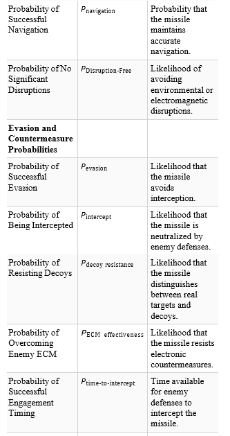
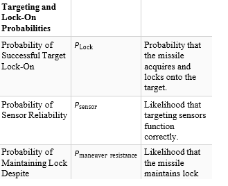
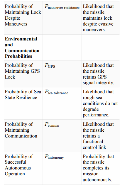
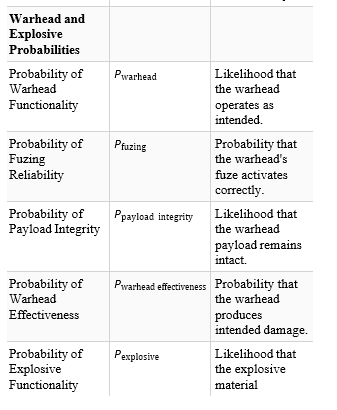
References

1. Huxley, T. H. (with University of California Libraries). (1869). On the physical basis of life. New Haven, Conn., The College Courant. http://archive.org/details/ onphysicalbasiso00huxlrich
2. Cale, J. (2018, October). Converging on Emergence: Reconnoitering to Optimally Adapt to Changes in System Environment. In 2018 IEEE International Systems Engineering Symposium (ISSE) (pp. 1-7). IEEE.
3. Gershenson, C. (2013). Facing complexity: Prediction vs. adaptation. In Complexity Perspectives on Language, Communication and Society (pp. 3-14). Berlin, Heidelberg: Springer Berlin Heidelberg.
4. Berry, B. J., Kiel, L. D., & Elliott, E. (2002). Adaptive agents,intelligence, and emergent human organization: Capturing complexity through agent-based modeling. Proceedings of the National Academy of Sciences, 99(suppl_3), 7187-7188.
5. Roach, J., Ewert, W., Marks, R. J., & Thompson, B. B. (2013, March). Unexpected emergent behaviors from elementary swarms. In 45th Southeastern Symposium on System Theory (pp. 41-50). IEEE.
6. Brinkmann, L., Cebrian, M., & Pescetelli, N. (2023). Adversarial dynamics in centralized versus decentralized intelligent systems. Topics in Cognitive Science.
7. Ferreira, E. D., Subrahmanian, E., & Manstetten, D. (2001, August). Intelligent agents in decentralized traffic control. In ITSC 2001. 2001 IEEE Intelligent Transportation Systems. Proceedings (Cat. No. 01TH8585) (pp. 705-709). IEEE.
8. Siqueira, L., & Abdelouahab, Z. (2006, April). A fault tolerance mechanism for network intrusion detection system based on intelligent agents (NIDIA). In The Fourth IEEE Workshop on Software Technologies for Future Embedded and Ubiquitous Systems, and the Second International Workshop on Collaborative Computing, Integration, and Assurance(SEUS-WCCIA'06) (pp. 6-pp). IEEE.
9. Torney, C., Neufeld, Z., & Couzin, I. D. (2009). Context- dependent interaction leads to emergent search behavior in social aggregates. Proceedings of the National Academy of Sciences, 106(52), 22055-22060.
10. Masek, M., Lam, C. P., Benke, L., Kelly, L., & Papasimeon,M. (2018, October). Discovering emergent agent behaviour with evolutionary finite state machines. In International conference on principles and practice of multi-agent systems (pp. 19-34). Cham: Springer International Publishing.
11. Reynolds, C. W. (1987, August). Flocks, herds and schools: A distributed behavioral model. In Proceedings of the 14th annual conference on Computer graphics and interactive techniques (pp. 25-34).
12. Weir, B. S., & Sokol, T. M. (2009, April). Radar coordination and resource management in a distributed sensor network using emergent control. In Defense Transformation and Net- Centric Systems 2009 (Vol. 7350, pp. 115-124). SPIE.
13. Linic, S., Lucanin, V., Zivkovic, S., Rakovic, M., & Puharic,M. (2020, June). Experimental and numerical methods forconcept design and flow transition prediction on the example of the bionic high-speed train. In International Conference of Experimental and Numerical Investigations and New Technologies (pp. 65-82). Cham: Springer International Publishing.
14. Sikdar, S., Rahman, M. H., Siddaiah, A., & Menezes, P. L. (2022). Gecko-inspired adhesive mechanisms and adhesives for robots—a review. Robotics, 11(6), 143.
15. Yu, Z., Zhang, H., Huang, J., Li, S., Zhang, S., Cheng, Y.,... & Lai, Y. (2021). Namib desert beetle inspired special patterned fabric with programmable and gradient wettability for efficient fog harvesting. Journal of Materials Science & Technology, 61, 85-92.
16. Wainwright, D. K., & Lauder, G. V. (2020). Tunas as a high- performance fish platform for inspiring the next generation of autonomous underwater vehicles. Bioinspiration & Biomimetics, 15(3), 035007.
17. Carijia, Z., Marušic, E., Novak, Z., & Fucak, S. (2014). Numerical analysis of aerodynamic characteristics of a bumped leading edge turbine blade. Engineering Review: Medunarodni casopis namijenjen publiciranju originalnih istrazivanja s aspekta analize konstrukcija, materijala i novih tehnologija u podrucju strojarstva, brodogradnje, temeljnih tehnickih znanosti, elektrotehnike, racunarstva i gradevinarstva, 34(2), 93-101.
18. Hapsari, F. N., Purwaningsih, R., Azzahra, F., & Sari, D. P. (2022, December). Velcro product design with biomimicry approaches. In IOP Conference Series: Earth and Environmental Science (Vol. 1111, No. 1, p. 012057). IOP Publishing.
19. Fontaine, S., Abbadie, L., Aubert, M., Barot, S., Bloor, J. M., Derrien, D., ... & Alvarez, G. (2024). Plant–soil synchrony in nutrient cycles: Learning from ecosystems to design sustainable agrosystems. Global Change Biology, 30(1), e17034.
20. Glabowski, M., Musznicki, B., Nowak, P., & Zwierzykowski,P. (2012). Shortest path problem solving based on ant colony optimization metaheuristic. Image Processing & Communications, 17(1-2), 7.
21. Lee, G. J., Yoo, Y. J., & Song, Y. M. (2018). Recent advances in imaging systems and photonic nanostructures inspired by insect eye geometry. Applied Spectroscopy Reviews, 53(2-4), 112-128.
22. Mandelbrot, B. B. (1995). Introduction to fractal sums of pulses. In Lévy Flights and Related Topics in Physics: Proceedings of the International Workshop Held at Nice, France, 27–30 June 1994 (pp. 110-123). Springer Berlin Heidelberg.
23. Bastos Filho, C. J., de Lima Neto, F. B., Lins, A. J., Nascimento, A. I., & Lima, M. P. (2008, October). A novel search algorithm based on fish school behavior. In 2008 IEEE international conference on systems, man and cybernetics (pp. 2646-2651). IEEE.
24. Eiben, A. E., & Smith, J. (2015). From evolutionary computation to the evolution of things. Nature, 521(7553), 476-482.
25. Leimar, O., & McNamara, J. M. (2023). Game theory ibiology: 50 years and onwards. Philosophical Transactions of the Royal Society B, 378(1876), 20210509.
26. Karmarkar, N. (1984, December). A new polynomial-time algorithm for linear programming. In Proceedings of the sixteenth annual ACM symposium on Theory of computing (pp. 302-311).
27. Anstreicher, K. M. (1999). Linear programming in O ([n3/ln n] L) operations. SIAM Journal on Optimization, 9(4), 803- 812.
28. Booker, A., Cramer, E., Frank, P., Gablonsky, J., & Dennis, J. (2007). Movars: Multidisciplinary optimization via adaptive response surfaces. In 48th AIAA/ASME/ASCE/AHS/ASC Structures, Structural Dynamics, and Materials Conference (p. 1927).
29. Seuken, S., & Zilberstein, S. (2005). Formal models and algorithms for decentralized control of multiple agents. Technical Report 05-68, Department of Computer Science, University of Massachusetts Amherst.
30. Bonabeau, E. (2002). Predicting the unpredictable. Harvard Business Review, 80, 109–116, 134.
31. Lodwick, W. A., & Untiedt, E. (2010). Introduction to fuzzy and possibilistic optimization. In Fuzzy Optimization: Recent Advances and Applications (pp. 33-62). Berlin, Heidelberg: Springer Berlin Heidelberg.
32. Hofman, R. (2006). Why Linear Programming cannot solve large instances of NP-complete problems in polynomial time. arXiv preprint cs/0611008.
33. Alidaee, B., Kochenberger, G. A., Lewis, K., Lewis, M., & Wang, H. (2009). Computationally attractive non-linear models for combinatorial optimisation. International Journal of Mathematics in Operational Research, 1(1-2), 9-19.
34. Fleck Jr, R. A. (1975). Computer efficiency and linearprogramming. The Computer Journal, 18(2), 115-116.
35. Ghadertootoonchi, A., Moeini-Aghtaie, M., & Davoudi,M. (2022). A hybrid linear programming-reinforcement learning method for optimal energy hub management. IEEE Transactions on Smart Grid, 14(1), 157-166.
36. O’Hare, G. M., O’Grady, M. J., Tynan, R., Muldoon, C.,Kolar, H. R., Ruzzelli, A. G., ... & Sweeney, E. (2007). Embedding intelligent decision making within complex dynamic environments. Artificial Intelligence Review, 27, 189-201.
37. Montreuil, B., & Laforge, A. (1992). Dynamic layout design given a scenario tree of probable futures. European Journal of Operational Research, 63(2), 271-286.
38. Li, Z., & Li, Z. (2016). Linear programming-based scenario reduction using transportation distance. Computers & Chemical Engineering, 88, 50-58.
39. Higle, J. L., & Wallace, S. W. (2003). Sensitivity analysis and uncertainty in linear programming. Interfaces, 33(4), 53-60.
40. Brown, G. G., Dell, R. F., & Wood, R. K. (1997). Optimization and persistence. Interfaces, 27(5), 15-37.
41. Branke, J. (2002). Optimization in dynamic environments. In Evolutionary Optimization in Dynamic Environments (pp. 13- 29). Boston, MA: Springer US.
42. Micacchi, C., & Cohen, R. (2006). A multi-agent architecturefor robotic systems in real-time environments. International Journal of Robotics & Automation, 21(2), 82.
43. Balmer, M., Nagel, K., & Raney, B. (2004, October). Large- scale multi-agent simulations for transportation applications. In Intelligent Transportation Systems (Vol. 8, No. 4, pp. 205- 221). Taylor & Francis Group.
44. Jha, S. S., & Nair, S. B. (2015). On a multi-agent distributed asynchronous intelligence-sharing and learning framework. In Transactions on Computational Collective Intelligence XVIII (pp. 166-200). Springer Berlin Heidelberg.
45. Berryman, A. A. (1992). The orgins and evolution of predator�prey theory. Ecology, 73(5), 1530-1535.
46. Abate, E. H., & Hofelich, F. (1969). An analytic solution of the Lotka Volterra equations. Zeitschrift für Naturforschung B, 24(1), 132-132.
47. Abdelkader, M. A. (1974). Exact solutions of Lotka-Volterra equations. Mathematical Biosciences, 20(3-4), 293-297.
48. Dahlin, M., Brooke, A., Narasimhan, M., & Porter, B. (2000). Data Synchronization for Distributed Simulations. In 2001 European Simulation Interoperability Workshop, SISO, Inc.,(CDROM) (pp. 25-27).
49. Hartley III, D. S. (1997, December). Verification & validation in military simulations. In Proceedings of the 29th conference on Winter simulation (pp. 925-932).
50. Ören, T. I. (2001, June). Impact of data on simulation: from early practices to federated and agent-directed simulations. In Proc. of EUROSIM (pp. 26-29).
51. Banos, A. (2010). La simulation à base d’agents en sciences sociales: une «béquille pour l’esprit humain 1»?. Nouvelles perspectives en sciences sociales, 5(2), 91-100.
52. Maldonado, G., & Greenland, S. (1997). The importance of critically interpreting simulation studies. Epidemiology, 8(4), 453-456.
53. Lewandowsky, S. (1993). The rewards and hazards of computer simulations. Psychological science, 4(4), 236-243.
54. Lüdtke, A., Möbus, C., & Thole, H. J. (2002). Cognitive Modelling Approach to Diagnose Over-Simplification in Simulation-Based Training. In Intelligent Tutoring Systems: 6th International Conference, ITS 2002 Biarritz, France and San Sebastian, Spain, June 2–7, 2002 Proceedings 6 (pp. 496- 506). Springer Berlin Heidelberg.