A Unified ISR World Model: Vossels, Voxels, Mipvols, and Reinforcement Learning

Introduction

Intelligence, Surveillance, and Reconnaissance (ISR) systems generate data from a wide spectrum of sources: electro-optical and infrared imagery, synthetic aperture radar, LiDAR point clouds, electronic emissions, cyber events, environmental fields, and multi-spectral or hyperspectral cubes. Each of these modalities arrives in a different structural form, rasters, volumes, tracks, signals, or logs, and are produced by sensors with unique geometries, resolutions, and statistical characteristics. Existing data structures handle these inputs in siloed ways: rasters are stored in grid-based formats, trajectories in tree indices, point clouds in unordered frames, and signals in time- frequency records. This fragmentation forces each modality into a heterogeneous pipeline, with separate methods for storage, indexing, subsampling, visualization, and fusion.

The result is inefficiency at multiple levels. At the computational level, data must be resampled or converted into secondary structures before joint analysis, incurring overhead and discarding fidelity. At the operational level, analysts are required to mentally reconcile disparate formats, shifting between images, tracks, and logs without a unified model of the environment. At the algorithmic level, reinforcement learning and other machine learning methods are forced to operate on reduced fidelity products, maps, tracks, or downsampled cubes, rather than the raw sensor measurements that carry the richest information content. These reductions are often irreversible, eliminating the anisotropy, blur, spectral spread, and uncertainty kernels that arise naturally from the physics of sensing.

Prior attempts at unification, such as temporal raster compression, trajectory indexing trees, or common point-cloud frames, have emphasized efficiency at the cost of fidelity. Compression schemes discard measurement geometry, point frameworks assume isotropy, and neural encoders abstract data into task-specific embeddings that no longer preserve the physical basis of observation. Format standards (e.g., HDF5, NGSI-LD, SensorML/O&M) improve interoperability but act as containers rather than representations, leaving the problem of how to capture the measurement itself unresolved.

The core problem, therefore, is the absence of a representation that simultaneously preserves raw sensor fidelity, supports efficient computation and memory management, and scales across heterogeneous ISR modalities. A solution would ideally unify sensing and non- sensing data within a consistent schema, maintain statistical and geometric detail, and remain tractable for real-time fusion, distributed processing, and AI exploitation. This is the gap that Vossels are designed to address.

Prior Work

Spatio-Temporal-Spectral Data Structures

Existing spatio-temporal data structures optimize for specific domains such as rasters, trajectories, or remote sensing imagery. Vossels differ by acting as a general abstraction: every sensor sample, regardless of type, is stored as a volumetric singular spectral element with spatial, temporal, and spectral attributes. This universality reduces the fragmentation of modality-specific data structures and creates a common foundation for fusion, interpolation, visualization, and AI-driven analysis. However, let us look in more detail.

The Temporal k²raster provides a compact representation and indexing method for temporal rasters [1]. The 2-3TR-tree extends this concept to trajectories of moving objects, supporting indexing of paths through continuous space [2]. A sliced representation model has been introduced to handle continuously changing spatial objects, partitioning them into temporal slices to capture evolution over time [3]. Adaptive tree structures have also been proposed that can dynamically switch between spatial and temporal indexing depending on query demands, improving efficiency under variable workloads [4]. More recently, spatio-temporal frameworks have been applied to problems such as clustering of space debris and spacecraft path optimization, demonstrating applicability in orbital dynamics and aerospace domains [5]. Parallel to these indexing methods, other work has focused on visualization and integration. Large wall displays have been used as a platform for handling video data in spatio-temporal form, while integrated storage structures have been designed for multi-dimensional remote sensing images to enable efficient retrieval across spectral and spatial dimensions [6,7]. Collectively, these methods are directed at the fundamental problem articulated by: the complexity inherent in representing, storing, and retrieving multidimensional data that evolves simultaneously in space, time, and spectral domains [8].

Let’s take a closer look at a few of the methods described above.

Temporal k²-Raster

The Temporal k²-raster provides a compressed structure for time-varying rasters, but it assumes a 2D grid and a single scalar per cell [1]. In contrast, Vossels generalize to full 3D volumes with multi-spectral channels and auxiliary attributes, enabling representation of volumetric sensor elements such as LiDAR beams or radar resolution cells rather than just raster pixels.

An extension, the temporal k²-raster (tk²r) is designed to manage time-varying raster datasets. It represents information as a hierarchy of rasters, each cell storing a single scalar value indexed by spatial position and time, expressed as R(x, y, t). This design is efficient for uniform gridded data such as land cover classification or temperature fields, where each sample is a homogeneous, single-valued measurement.

Vossels differ in both structure and scope. A Vossel is defined as an atomic record in the space where (x, y, z) are spatial coordinates, t is time, {λi} are spectral channels, and {aj} are auxiliary attributes such as amplitude, polarization, or classification confidence. Each Vossel therefore represents not just a raster cell value but a multi-dimensional, modality-agnostic sample that can encode the geometry, variance, and physical observables of a sensor measurement.

This distinction has several implications. First, tk²r assumes a 2D raster base, whereas Vossels natively extend into three-dimensional volumes, allowing representation of LiDAR point clouds, volumetric SAR cells, or acoustic lobes. Second, tk²r stores a single scalar per cell, while Vossels can carry full spectral vectors and metadata attributes. Finally, tk²r is tied to regular grids, whereas Vossels act as unifying containers that can accommodate heterogeneous ISR modalities—optical pixels, radar resolution cells, SIGINT emissions, jamming fields, or cyber events—within the same structure.

Although useful, tk²r is optimized for uniform raster streams, while Vossels generalize to heterogeneous, high-dimensional ISR data. This generalization allows all sensing and non-sensing inputs to be stored in one consistent framework, enabling fusion, interpolation, and reinforcement learning over datasets that would otherwise remain siloed.

2-3TR-Tree

The 2-3TR-tree was introduced to manage spatio-temporal trajectories by extending balanced search tree concepts into the temporal domain [2]. Each node maintains bounding rectangles over spatial extents coupled with temporal intervals, allowing efficient queries such as “which trajectories pass through region R during [t0, t1]?”. Insertions and deletions are handled dynamically, making the 2-3TR- tree suitable for databases where objects move continuously and queries require path retrieval, intersection tests, and spatio-temporal joins. Its design emphasizes efficient indexing of P(t) = (x(t), y(t)) paths, typically with a small number of attributes beyond position.

Vossels diverge from this design in several fundamental ways. First, the 2-3TR-tree treats trajectories as first-class entities and compresses motion into linked path segments. By contrast, Vossels preserve each raw measurement with allowing full volumetric representation and λi , aj encoding spectral and auxiliary attributes such as polarization, amplitude, confidence, or modulation. This distinction enables Vossels to capture not just the path of an object, but also its evolving physical observables across modalities.

Second, while the 2-3TR-tree is efficient for point-like trajectories, it is not designed for measurements that extend spatially, such as radar resolution cells, LiDAR beam footprints, or EO pixels. Vossels explicitly include projected geometry and statistical kernels, which allows anisotropic and blurred sensor footprints to be represented as probability distributions within a voxel volume. This feature is critical for ISR data, where sensing rarely yields perfect point measurements.

Finally, in terms of computational scope, the 2-3TR-tree is bounded by the requirements of trajectory indexing and retrieval. Vossels generalize this by enabling not only motion queries but also fusion, interpolation, and learning. A moving object is represented as a sequence of Vossels that can be grouped into voxels, accumulated into mipvol hierarchies, and queried via frustum extraction. This al- lows the same data to support both classical trajectory queries and advanced reinforcement learning tasks, where the agent must reason over evolving spatial signatures, temporal correlations, and multi-modal observables.

While the 2-3TR-tree provides an efficient indexing structure for trajectory databases, it is tied to position-centric representations. Vossels expand the abstraction to full volumetric, spectral, and attribute-rich measurements, enabling multi-modal exploitation and AI- driven analysis.

Sliced Representation Models

The sliced representation model addresses temporal change by storing spatial objects as a sequence of slices, each slice representing the geometry at a particular time step [3]. Continuity is enforced by linking successive slices, which enables queries over discrete states such as the geometry of an object at time t or its transformation between t0 and t1. This design is effective for surface-based or polygo- nal objects whose changes can be approximated as a series of snapshots, but it requires resampling all data into aligned temporal layers.

The limitation of this approach is that it assumes regular updates and bounded geometries, which does not reflect the irregular, asynchronous, and heterogeneous character of ISR data. Sensors rarely align to a common temporal grid, and their measurements often include uncertainty, blur, or probabilistic boundaries that cannot be easily expressed as crisp surfaces in slices.

By contrast, the Vossel framework avoids fixed temporal layering and instead supports continuous temporal evolution through direct incorporation of time into its volumetric-spectral schema. Rather than maintaining geometry in discrete snapshots, measurements are organized hierarchically into voxels and mipvols for efficient binning, retrieval, and interpolation. This preserves irregular sensor timing and allows data fusion across modalities without forcing artificial synchronization. Sliced models provide continuity across discrete frames, whereas Vossels enable scalable continuity across both time and modality in a unified representation.

Adaptive Tree Structures

Adaptive tree structures attempt to balance spatial and temporal indexing by dynamically switching between them based on query type [4]. For example, queries constrained in time may favor temporal indexing, while spatial queries rely on partitioning the data domain into regions or cells. This adaptability improves performance for workloads that shift between spatial and temporal dominance, but it requires the system to continuously monitor query patterns and restructure indices.

The weakness of this approach is that it still relies on rigid indexing strategies tied to either space or time as primary keys. ISR data is not easily reduced to such partitions, since it contains spectral vectors, auxiliary observables, and probabilistic kernels that span beyond simple spatio-temporal ranges. Adapting tree nodes can mitigate some inefficiencies, but the data remains locked into point or cell ab- stractions with limited extensibility.

Vossels extend beyond this paradigm by incorporating space, time, and spectrum simultaneously at the atomic level. Organizational structures such as voxels and mipvols are applied secondarily, not as the primary indexing basis. This duality of atomic records and volumetric grouping enables efficient memory management and distributed computation while preserving the multidimensional richness of the original measurement. Adaptive trees improve query flexibility within spatio-temporal domains, but Vossels provide a foundation where fusion, interpolation, and learning can occur across modalities without being bound to tree restructuring.

Spatio-Temporal indexing

Applications in space debris clustering and path optimization demonstrate the utility of spatio-temporal indexing for specialized domains [5]. Vossels provide a broader foundation: instead of task-specific indexing, they unify all ISR modalities—including imagery, radar, SIGINT, jamming, and cyber—into one structure that supports both trajectory-style queries and spectral fusion.

Applications-Oriented Structures

A number of spatio-temporal-spectral data structures have been built for specific workloads. Space-operations frameworks target orbital trajectories and collision risk, tuning indexes to predictive clustering and path optimization [5]. For high-throughput media and remote sensing, virtual large wall displays emphasize tiled, parallel playback of video streams, while integrated multi-dimensional image stores organize remote-sensing cubes with chunked tiling, pyramid levels, and metadata indexes to accelerate read-heavy raster analytics [6,7]. These systems show clear performance wins but share two traits: they assume regular grids (or tightly controlled tiling) and require modality-specific adaptation when data deviates from uniform rasters.

Samet’s survey frames the indexing landscape—quadtrees, k-d trees, and higher-dimensional variants extended into time—prioritizing compression and query cost over preservation of measurement physics [8]. That abstraction is geometric and algorithmic, not semantic.

Vossels extend these ideas without inheriting their constraints. They retain raw observables (including anisotropy and uncertainty) and then layer voxels/mipvols for scalable storage and query, rather than forcing all inputs into uniform rasters or tiles. As a result, the same store supports reinforcement-learning policies and automated fusion across imaging, radar, LiDAR, SIGINT, cyber, and environmental feeds—combining fidelity preservation with computational efficiency in distributed or heterogeneous ISR environments.

Unifying Data Structures

Attempts at unifying spatio-temporal-spectral data structures can be grouped into three broad categories. The first category is volumetric stores, such as voxel grids, octrees, and their multi-resolution derivatives. These approaches are effective for spatial partitioning and memory efficiency, particularly when handling large image stacks, LiDAR scans, or SAR volumes, and they enable hierarchical querying. However, they require all incoming samples to be discretized into a fixed volumetric lattice. This resampling erases the native footprint, anisotropy, and statistical properties of the original measurements, reducing their utility for estimation-theoretic operations.

The second category is common point-cloud frames, which express heterogeneous sensor inputs as sets of 3D points with associated attributes. These frames facilitate alignment and registration across modalities and are widely used in robotics and geospatial pipelines. Extensions such as probabilistic projection maps and semantic voxel representations attempt to capture uncertainty and classification information. Yet point-based abstractions generally assume isotropic samples and do not encode blur, coherence, or spectral spread. Their memory footprint also grows rapidly without aggressive compression or clustering, making them less practical for ISR-scale data.

The third category is modality-agnostic neural encoders, where raw sensor data are projected into shared feature embeddings using learned networks [6,7]. This provides flexibility for classification, detection, and cross-modal reasoning, as the representation is automatically adapted to downstream tasks. However, embeddings abstract away the physical basis of the measurement. Once converted, the original footprint, point spread function, and spectral fidelity are lost. This limits their use in physically grounded fusion and estimation, or in reinforcement learning contexts where raw observables provide richer training signals.

Format Standards

A parallel line of work has pursued format and interoperability standards, includ-ing HDF5 for structured multi-dimensional storage, NGSI-LD for linked data integration, and SensorML/O&M for metadata and sensor descriptions. LLVM-inspired intermediate forms have been proposed to improve modularity and transformation pipelines. These standards reduce friction between systems and enable scalable data exchange, but they act primarily as containers rather than unifying representations. Like the categories above, they achieve efficiency or interoperability by forcing all measurements into uniform points, cells, or embeddings, thereby stripping away much of the richness that originates in the sensor physics.

Vossel Distinction

Vossels extend beyond these approaches by retaining the atomic measurement with its projected geometry, statistical kernel, anisotropy, and spectral attributes, embedding it directly into volumetric and temporal context. Unlike voxel and octree methods, they do not rely on a single discretization but allow aggregation into voxel bins and mipvol hierarchies as secondary organizational layers. Unlike point- cloud frameworks, they encode polarization, coherence, and uncertainty rather than assuming isotropy. Unlike neural encoders, they unify modalities without discarding raw fidelity or requiring task-specific retraining. Finally, unlike format standards, they constitute a mathematically grounded representation rather than a passive container.

The duality of storage—raw spectral elements organized into volumetric hierarchies—provides computational efficiency and scalable memory management independent of GPU versus CPU execution. This design enables distributed and cluster computing, with voxel binning and mipvol hierarchies supporting efficient query and adaptive fidelity. The result is a framework that preserves the richness of sensor physics while remaining computationally tractable at ISR scale, and that directly supports reinforcement learning agents and automated fusion methods operating over heterogeneous, high-dimensional inputs.

Structure	Domain	Representation	Strengths	Limitations	Vossel Contrast
Temporal	2D rasters over	Hierarchy of	Compact,	Limited to 2D,	Vossels generalize
k²raster	time	rasters, one scalar	efficient for	single scalar,	to
(Cerdeira-Pena et al. 2018)		per cell R(x, y, t)	uniform grids	assumes homogeneity	(x, y, z, t, λi, aj) , capturing 3D,
					multispectral, and
					auxiliary
					attributes with
					variance
2-3TR-tree	Moving objects	Spatio-temporal	Efficient	Restricted to	Vossels encode
(Abdelguerfi et al.		tree combining 2-	trajectory	discrete path	full sensor
2002)		and 3-way	indexing and	storage; does not	samples
		branching	retrieval	capture	(geometry, PSF,
				measurement	spectral spread)
				physics	rather than just
					paths
Sliced	Continuously	Sequential slices	Maintains	Inherits	Vossels model
representation	changing spatial	of object states	continuity over	discretization	continuous
(Forlizzi et al.	objects		time	artifacts;	distributions via
2000)				unsuitable for	kernels,
				high-dimensional	preserving
				ISR	anisotropy and
					spectral detail
Visualization and	Video walls,	High-	Optimized for	Limited to	Vossels combine
storage (Wang et	remote sensing	performance	human use and	rasterized video	visualization with
al. 2003; Zhang et	images	visual and multi-	imagery	or image cubes	mathematically
al. 2017)		dimensional			grounded
		image access			representation,
					enabling fusion
					and RL across
					modalities
Vossels	ISR multi-modal	Volumetric	Preserves sensor	Higher storage	Provides
		singular spectral	fidelity; supports	requirements than	universal,
		elements	fusion, scalable	compressed	physically
		(x, y, z, t, λi, aj )	memory	schemes;	grounded
		+ voxel/mipvol	management, RL	emphasizes	abstraction across
		hierarchy	integration	fidelity over compression	ISR modalities

Comparitive Analysis

Prior spatio-temporal-spectral data structures have emphasized indexing, com-pression, or specialized representations for efficiency. The Temporal k²raster achieves compact representation of time-varying rasters but is limited to uniform 2D grids with a single scalar per cell, optimized for homogeneous raster streams such as temperature or land cover fields [1]. The 2-3TR-tree was designed to index moving object trajectories by combining two- and three-way branching factors, enabling efficient retrieval of discrete paths but offering little support for continuous measurement geometry or multi-modal fusion [2]. Sliced representation models attempt to preserve continuity of spatial objects across time by storing sequential “slices” of state, but they inherit discretization artifacts and are poorly suited to heterogeneous, high-dimensional ISR modalities [3]. Other work has emphasized visualization and storage, such as virtual large wall displays for video data and integrated multi-dimensional storage structures for remote sensing images [6,7]. These approaches provide high-performance access for specialized im-agery but remain tied to rasterized or modality-specific forms.

Whereas these structures optimize for specific data types—rasters, trajectories, videos, or image cubes—Vossels act as a universal abstraction. Each measurement, whether optical, radar, LiDAR, SIGINT, cyber, or environmental, is represented as a volumetric singular spectral element with spatial, temporal, spectral, and auxiliary attributes. This reduces fragmentation across modalities, simplifies fusion, and provides a consistent basis for reinforcement learning and adaptive ISR analysis. Unlike voxel and octree methods, Vossels are not bound to a fixed discretization: voxel bins and mipvol hierarchies are applied only as secondary organizational structures, leaving the atomic measurement intact. Unlike pointcloud frameworks, they do not assume isotropy but explicitly preserve anisotropy, coherence, blur, polarization, and spectral spread. Unlike neural encoders, they unify modalities without discarding raw fidelity or requiring retraining on task-specific embeddings. Finally, unlike passive container standards such as HDF5, NGSI-LD, or SensorML/O&M, Vossels constitute a mathematically grounded representation that retains the physics of the sensing process.

This distinction is operationalized by embedding atomic spectral elements directly into volumetric and temporal context, while applying statistical kernels, view frustum extraction, kriging interpolation, and multiresolution mipvol hierarchies to manage data adaptively. By retaining the projected geometry and uncertainty kernel of each measurement, Vossels maintain the dual representation of geometric footprint and statistical variance. This allows heterogeneous inputs to be normalized into a single data model while preserving the physics of collection. In practice, this means that radar resolution cells, optical pixels, LiDAR beams, acoustic lobes, SIGINT emissions, cyber events, and environmental fields can all be ex-pressed within the same structure, consistently aligned and fused.

The dual structure—atomic Vossels embedded within voxel and mipvol hierarchies—provides computational efficiency and scalable memory management independent of CPU versus GPU execution. Voxels serve as spatial bins that cluster measurements for locality of reference, while mipvols provide multiresolution detail management, ensuring that queries and visualization operate only at the reso- lution required. This design enables intrinsic reduction without discarding raw measurements: high-level tasks can exploit voxel-level aggregates, while precision analysis reverts to the underlying Vossels. On CPUs, voxel binning accelerates cache coherence; on GPUs, mipvol subsampling reduces VRAM demand; and in distributed settings, voxel partitions map naturally across clustered environments. The result is a fidelity-preserving yet computation-aware framework suitable for ISR exploitation at scales ranging from embedded platforms to global clusters.

Vossels and Reinforcement Learning

Reinforcement learning benefits directly from this design. Agents can exploit the voxel–mipvol hierarchy for curriculum training, beginning with coarser mipvol levels to learn policies over large-scale patterns before refining them on raw Vossel data. This reduces training time, provides natural hierarchical policy development, and eliminates the need for external resampling. By contrast, structures such as the Temporal k²raster or trajectory trees achieve efficiency primarily through compression and indexing, forcing simplification into uniform rasters or trajectory records. Vossels avoid this reduction, preserving the underlying measurement physics while still enabling scalable management. This makes them well suited for reinforcement learning agents that require rich, high-dimensional inputs and consistent semantics across sensing domains.

Vossels also provide significant advantages beyond reinforcement learning. They act as hyperdimensional state elements in which spatial coordinates, temporal attributes, modality-specific measurements, environmental modifiers, degraders, and uncertainty descriptors are co-embedded in a unified structure. Each Vossel is therefore a pre-normalized representation, ensuring that all channels are inherently aligned in the same coordinate system and update cycle. This removes the need for extensive preprocessing, including normalization, co- registration, and cross-modal alignment, which is required in conventional ISR pipelines. The result is reduced computational overhead, lower latency, and direct applicability for machine learning and spiking architectures.

A major benefit of this unified design is that analytic operations need not be performed on fragmented or separately conditioned products. Segmentation, recognition, correlation, and prediction operate directly on the Vossel substrate, which is already fused and semantically coherent. This prevents errors that arise when sub-systems attempt to reconcile outputs that were produced under inconsistent as- sumptions. It also allows reinforcement learning agents to operate on data that is physically grounded, temporally consistent, and enriched with environmental and degradative context.

Another advantage is that Vossels encode degraders and environmental factors alongside direct sensor returns. Jamming, cyber-induced network degradation, atmospheric absorption, scattering, diffusion, and weather are not handled externally but are represented as explicit channels within the same compositional framework. Updates to these channels condition observations in place, reducing sensor confidence or modifying likelihoods locally rather than requiring separate bookkeeping. This integration produces a more resilient operational model: when one modality is compromised, other modalities are weighted accordingly, and confidence is adjusted without external intervention.

The structure also facilitates adaptive resolution management. Coarser mipvols allow global context to be preserved, while raw Vossels maintain the full measurement physics for finegrained exploitation. This hierarchy ensures that both reinforcement learning agents and analytic processes can scale from broad situational understanding to detailed forensic analysis without abandoning the common substrate. In practice, this improves training efficiency, supports multiscale optimization, and ensures continuity between coarse decision-making and finegrained evidence.

Vossels extend beyond compression or indexing to provide a universal, physically grounded abstraction for ISR. They preserve raw sensor fidelity, capture environmental and degradative effects in the same representational space, support adaptive multiresolution storage, and enable reinforcement learning and automated fusion methods over heterogeneous, high-dimensional data. By shifting emphasis from storage efficiency alone to a representation optimized for fusion, adaptability, and AI-driven exploitation, Vossels provide broader operational capability and a more direct path from sensing to decision than any prior spatio-temporal-spectral structure.

Vossel Design

ISR sensor data originates across the electromagnetic spectrum and may be expressed in the form of points, images, or depth maps depending on the modality. Each sensor operates at a different target or ground resolution, and therefore the resulting measurements are heterogeneous in scale. To preserve fidelity, the system stores the data at full native resolution. However, subsequent analytical or visualization tasks do not always require this level of detail, and so the data can later be retrieved at an appropriate resolution. Because many applications require efficient access to neighboring measurements, the data must be organized in a clustered fashion that facilitates local searches.

The measurements collected by each sensor are not uniform in their structure. In addition to spatial position, described by (x, y, z) coordinates, a sample may include amplitude, polarization, color, phase, spectral shift, or other physical observables, and each record carries a time stamp t. Thus, an individual measurement is represented as a Vossel:

                                                          v = x, y, z, t, λ1, … , λn, a₁, … , a_m,

where λ_i denotes the spectral bands and a_j the auxiliary attributes.

Before the data is integrated into a common framework, each sensor feed is subjected to preprocessing steps. These include sensor- specific geometric and photometric corrections, amplitude normalization, and local operations such as gamma correction and sharpening. Once normalized, the feeds are routed into the Vossel Integrator, which performs single-channel mosaic buildup, multichannel registra- tion, warping, rectification, and ultimately aggregation into the world model state.

As part of this integration, the data is binned into voxels to provide a computational grouping mechanism. A voxel is defined as

                       V_i,j,k = [x₀ + iΔx,, x₀ + (i + 1)Δx) × [y₀ + jΔy,, y0 + (j + 1)Δy) × [z₀ + kΔz,, z₀ + (k + 1)Δz),

with i, j, k indexing the grid. Each Vossel belongs uniquely to one voxel:

                                                              ∀v ∈ E ,; ∃(i, j, k) : (x, y, z) ∈ V_i,j,k.

These voxels are further organized into mipvol hierarchies, enabling multiresolution access. Because each Vossel is time stamped, data can be accumulated into a single voxel structure and then segmented into time-series voxel volumes. The segmentation interval is application-defined: for low-volume sensors, a time slice may represent one minute, whereas for high-volume sensors, one second slices are more appropriate. A time-sliced voxel set is therefore:

                                                                 V[t0, t1] = v ∈ E | t0 ≤ t ≤ t₁.

When analysis or visualization is required, a frustum extractor defines the selection of voxels or mipvols from the world model. A frustum query F with near plane h and far plane y extracts:

                                                      F(F , [t₀, t₁]) = v ∈ E | (x, y, z) ∈ F ,; t₀ ≤ t ≤ t₁.

    The fidelity of this extraction can be adapted to the performance requirements of the task. For low-performance, low-fidelity applications, Vossels may be used directly as statistical representations of voxels, i.e.,

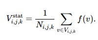
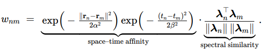
For high-fidelity operations, kriging interpolation is applied to estimate desired values at specific coordinates (x, y, z, t):

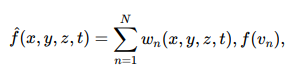
with weights wn determined by the spatial–temporal covariance model.

The degree of granularity is also adjustable during frustum extraction. Typically, lower resolution mipvol levels are used for regions that are farther from the hither plane, with higher resolution reserved for the near field. Yon planes may be set to limit the overall data volume or may be defined adaptively, either globally or on a per-channel basis, depending on the deterioration of signal-to-noise ratio with distance.

Through this sequence of operations, ISR data is transformed from heterogeneous sensor feeds into a coherent world model that can be queried at appropriate temporal and spatial scales. The combination of formal primitives (Vossels), organizational structures (voxels, mipvols), and extraction operators (frustum selection, kriging interpolation) provides both efficiency and adaptability, ensuring that analysis and visualization tasks can operate on the resolution and fidelity best suited to the mission requirements.

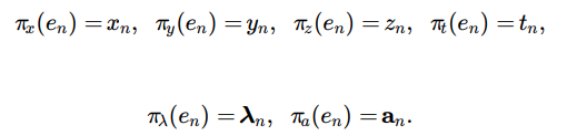
vossel Definition

A Vossel (Volumetric Singular Spectral Element) is an atomic spatio-spectral-temporal sample with real-world coordinates and associated footprint and uncertainty, which we can define as:

                               e_n = ( p_n, F_n, Σ_n, λ_n, a_n ),

where

- p_n = (x_n, y_n, z_n, t_n) ∈ D × T is the nominal space–time center,

- Fn ⊂ R³ is the projected footprint envelope (deterministic support),

- Σ_n is a positive semidefinite kernel/covariance describing spatial (and optionally temporal/spectral) uncertainty,

- λn ∈ R^Bn is the spectral vector (possibly band-dependent length B_n ),

- an ∈ R^Mn collects auxiliary attributes (e.g., intensity, phase, polarization, SNR, class/confidence).

This definition preserves the dual nature of a measurement: F captures determinis-tic footprint geometry, Σ and captures stochastic variance around it.

Structural Relationships

The Vossel is defined as the atomic sensing element, but its utility emerges only when it is related to higher-order organizational structures. The voxel grid provides the discretized support in which Vossels are embedded. Defined over a spatial domain with fixed origin and cell sizes, the voxel grid partitions space into half-open volumes, ensuring that the domain of interest can be exhaustively covered by a finite set of cells. This provides the scaffolding for indexing and aggregation without requiring that the raw measurements themselves be resampled.

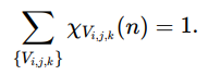
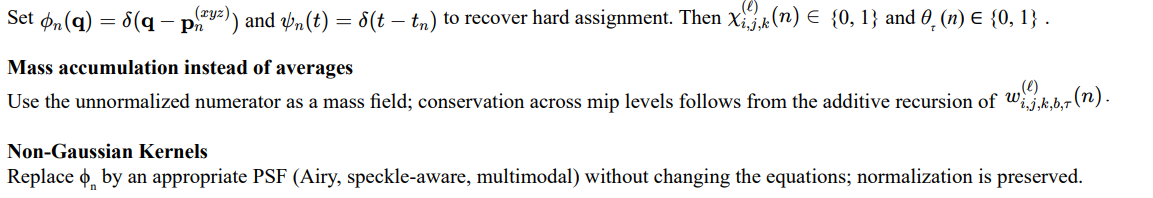
The element set ∈ is the collection of all Vossels in the scene, each carrying its spatio-temporal position, footprint, uncertainty kernel, and spectral attributes. These elements are positioned continuously in space, but for computational tractability they must be assigned to discrete bins in the grid. The element–voxel assignment formalizes this step: each Vossel is mapped deterministically to a voxel by integer division of its coordinates relative to the grid origin and cell sizes. This produces a one-to-one containment when variance is negligible, but more generally requires a probabilistic assignment when the uncertainty kernel spans multiple cells.

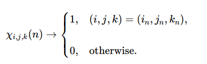
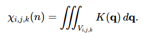
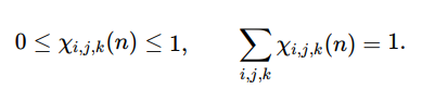
The probabilistic assignment leads directly to the definition of occupancy. Rather than a binary indicator, the fractional occupancy χi,j,k (n) is computed by integrating the Vossel’s uncertainty kernel over the voxel volume. In the limit of negligible variance this reduces to 0 or 1, but when the Vossel footprint overlaps several cells the occupancies act as weights distributed across them. The triple-sigma oc- cupancy ensures conservation by guaranteeing that the sum of weights across all voxels for a given Vossel equals one, thereby preserving the total element count under probabilistic spreading.

Self-containment follows as a consistency condition. Provided that the voxel grid covers the sensing domain, the set of all Vossel centers lies within the union of voxel supports, and for every element there exists at least one cell containing it. This ensures that the voxelized representation is complete and that no measurement is lost or discarded in the embedding process.

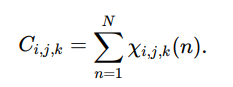
Aggregation over voxels extends this containment by allowing functions of the elements to be accumulated cell by cell. Any per-element attribute—such as amplitude, polarization energy, or classification score—can be summed within a voxel using the occupancy weights. Conservation identities guarantee that the global sum of any attribute over all Vossels equals the sum over all voxel aggregates, ensuring exactness and enabling efficient reduction operations.

A multiresolution hierarchy, or mipvol construction, generalizes the grid into a pyramid of scales. By doubling the voxel size at each level, parent volumes subsume the contents of their children while maintaining strict count consistency. This allows adaptive fidelity: queries can be answered coarsely at high levels or precisely at the base resolution, and reinforcement learning can exploit coarse-to- fine training curricula. The dual representation, atomic Vossels preserved in continuous space, organized hierarchically into voxels and mipvols, creates a framework that is simultaneously fidelity-preserving, computationally efficient, and scalable across hardware architectures.

Voxel Grid

Let the spatial domain be D ⊂
 with origin (x₀ , y₀, z₀ ). 

Fix cell sizes Δx, Δy , Δz > 0 and extents N _x ,N_y , N_z ∈
> 0.

Definition of a voxel

A voxel (half-open cuboid cell) is

                V_i,j,k = [x₀ + iΔx, x₀ + (i + 1)Δx) × [y₀ + jΔy, y₀ + (j + 1)Δy) × [z₀ + kΔz, z₀ + (k + 1)Δz),

with integer indices

                                       i ∈ [0, N_x − 1], j ∈ [0, N_y − 1], k ∈ [0, N_z − 1] ∩ Z.

The collection of all voxels partitions the grid support:

By construction, the voxels are disjoint except at boundaries:

                    V_i,j,k ∩ V_i′,j′,k′ = ∅ if (i, j, k) f= (i′, j′, k′).

Indexing Map

Define the index map : D →  by

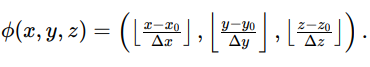
For any point r = (x, y, z) ∈ D, (r) = (i, j, k) yields the voxel index such that r ∈ V_i,j,k .

This mapping is surjective onto the voxel index set {0,…,N_x − 1} × {0,…,N_y − 1} × {0,…,N_z − 1} .

Volume and Centroid

The volume of a voxel is constant:

                                             Vol(V_i,j,k) = Δx Δy Δz.

The centroid is

                                         c_i,j,k = (x0 + (i + ½ )Δx, y0 + (j + 1 )Δy, z0 + (k + ½ )Δz).

These centroids form a lattice of points embedded in D.

Indicator Functions 

Define the indicator of voxel membership:

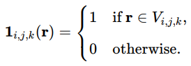
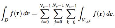
Then any measurable function f : D →
can be decomposed as

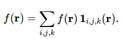
Integration reduces to

Voxel Occupancy (Counts)

Given an element set∈= {e_n} with positions r_n = (x_n, y_n, z_n), define the voxel count

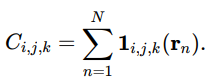
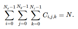
Conservation identity:

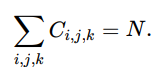
In the probabilistic case with soft occupancies χ _i,j,k (n) ∈ [0, 1] , the generalized count is

Non Cartesian Voxel Domains

Voxels need not be restricted to Cartesian lattices. Certain classes of problems are better expressed in alternate domains such as Fourier space, spherical–polar coordinates, or other non-Euclidean geometries. In general form, a voxelized field can be defined as a mapping

                                                                    V : Ω → Rⁿ

where Ω is a discrete sampling of a continuous manifold M equipped with a coordinate metric g. The metric determines the adjacency and locality relations among voxels. For standard volumetric grids, M = R³ and g is Euclidean, but this is only a special case.

In Fourier space, the voxel indices correspond to frequency coordinates (k_x, k_y, k_z), and the field V (k_x , k_y , k_z) encodes spatial frequency amplitude and phase rather than position. This formulation is advantageous for convolution, filtering, and correlation, where differential operators become multiplicative.

In spherical or polar voxelizations, the coordinates are expressed as (r, θ, ), and the discretization is uniform in angular rather than linear space. Such arrangements are efficient for radiance fields, omnidirectional sensing, or any geometry exhibiting radial symmetry.

More generally, non-Cartesian lattices can be defined on curvilinear or manifold-adapted spaces, such as cylindrical (r, , z), log-polar, or geodesic grids. These support applications in flow visualization, astronomical mapping, and imaging where anisotropy or curvature makes uniform Euclidean sampling inefficient.

Under this view, a voxel is simply a discrete tensor element defined over an arbitrary coordinate manifold, with topology and neighborhood structure inherited from g. The voxel concept therefore extends naturally to any domain where continuity and adjacency can be formalized, independent of whether the underlying space is Cartesian, spectral, or curved.

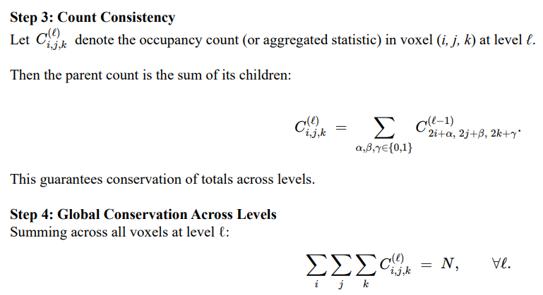
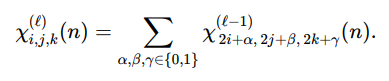
Multiresolution Hierarchy

<img src=" https://www.opastpublishers.com/scholarly-images/9912-691db1bd888bf-a-unified-isr-world-model-vossels-voxels-mipvols-and-reinfor.png" width="500" height="200">

Thus, total conservation holds at every level:

<img src=" https://www.opastpublishers.com/scholarly-images/9912-691db2245c8a3-a-unified-isr-world-model-vossels-voxels-mipvols-and-reinfor.png" width="200" height="100">

The voxel grid provides a partition of space into uniform volumetric bins with explicit index mapping, centroid locations, indicator functions, and count conservation. By embedding Vossel elements into this grid, either deterministically via index maps, or probabilistically via kernelized occupancies, it becomes possible to aggregate, query, and downsample measurements while preserving global consistency. The multiresolution extension forms the basis of mipvol hierarchies (more on this later), ensuring scalable representation across CPU, GPU, and distributed architectures.

Element Set

Let the spatial domain be D ⊂ R³ and time domain T ⊂ R.

As a reminder, a Vossel is an atomic sample

                               e_n = ( p_n, F_n, Σn, λ_n, a_n ),

where

- p_n = (x_n, y_n, z_n, t_n) ∈ D × T is the nominal space–time center,

- F_n ⊂ R³ is the projected footprint envelope (deterministic support),

- Σn is a positive semidefinite kernel/covariance describing spatial (and optionally temporal/spectral) uncertainty,

- λn ∈ R^Bn is the spectral vector (possibly band-dependent length B_n ),

a_n ∈ R^Mn collects auxiliary attributes (e.g., intensity, phase, polarization, SNR, class/confidence)

The element set is

<img src=" https://www.opastpublishers.com/scholarly-images/9912-691db400c888e-a-unified-isr-world-model-vossels-voxels-mipvols-and-reinfor.png" width="200" height="100">

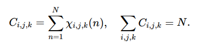
Coordinate and Attribute Projections

Define projection maps:

Concatenate r_n = (x_n, y_n, z_n) and pn = (r_n, t_n).

Empirical Measures Over Space Time and Spectrum

The empirical space–time measure of centers:

<img src=" https://www.opastpublishers.com/scholarly-images/9912-691db591e3a80-a-unified-isr-world-model-vossels-voxels-mipvols-and-reinfor.png" width="200" height="100">

with δ_pn the Dirac at pn.

If a per-element nonnegative weight w_n (e.g., quality, confidence) is available:

<img src=" https://www.opastpublishers.com/scholarly-images/9912-691db5d83be0d-a-unified-isr-world-model-vossels-voxels-mipvols-and-reinfor.png" width="200" height="100">

For a fixed band index b (or spectral response R_b):

<img src=" https://www.opastpublishers.com/scholarly-images/9912-691db626e6294-a-unified-isr-world-model-vossels-voxels-mipvols-and-reinfor.png" width="500" height="100">

Kernelized Occupancy (soft presence in a region)

Let Kn (⋅ ; p_n, Σ_n) be the normalized spatial kernel induced by Σ_n around r_n.

For any region A ⊂ D:

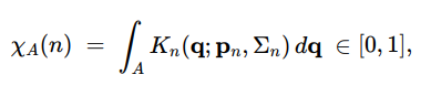
with partition of unity

This reduces to a hard indicator when Σ_n → 0 and F_n ⊂ A.

Neighborhoods and Selection Sets

Given a query p₀ = (r₀, t₀) and selection parameters

                           ρ > 0 (spatial radius), τ > 0 (temporal half-width), F ⊂ D (view frustum),

define the neighbor index set

                                     N (p₀; ρ, τ , F ) = { n : r_n − r₀ ≤ ρ, |t_n − t₀| ≤ τ , r_n ∈ F }.

A band/material filtered neighborhood is

                                          N_b,m = {n ∈ N : b ∈ e_n, m_n = m},

where m_n is an optional material label.

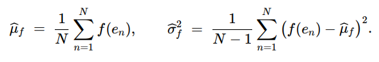
Empirical Moments (per band or attribute)

For a scalar per-element function f (e_n):

Over a neighborhood N

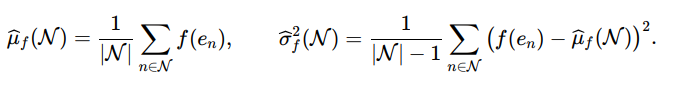
For multiband vectors λ_n ∈ R^B:

<img src=" https://www.opastpublishers.com/scholarly-images/9912-691e929d909ae-a-unified-isr-world-model-vossels-voxels-mipvols-and-reinfor.png" width="500" height="100">

Cross Covariances (space time vs. spectrum)

Let g (p_n) be a scalar function on space–time and h (λ_n) a scalar spectral function

<img src=" https://www.opastpublishers.com/scholarly-images/9912-691e92f0c13b0-a-unified-isr-world-model-vossels-voxels-mipvols-and-reinfor.png" width="500" height="100">

This quantifies coupling useful for co-kriging or feature selection.

Element Graphs (for fusion/association)

Define a proximity graph G = (V , E) with V = {1,…, N} and

                           (n, m) ∈ E ⇔ ||r_n − r_m|| ≤ ρ_s,|t_n − t_m|≤ ρt.

Optionally weight edges by similarity

<img src=" https://www.opastpublishers.com/scholarly-images/9912-691e93d835558-a-unified-isr-world-model-vossels-voxels-mipvols-and-reinfor.png" width="500" height="100">

This graph supports track-building, clustering, and factor-graph fusion.

Element Level Likelihoods

Given a forward model M producing expected attribute fθ (p, λ) with parameter θ and noise covariance Σ_n :

This leads to MAP/ML estimators θ^ and uncertainty propagation over ε

Element Histograms and Densities

<img src=" https://www.opastpublishers.com/scholarly-images/9912-691e95bfe5206-a-unified-isr-world-model-vossels-voxels-mipvols-and-reinfor.png" width="500" height="100">

Kernel density estimate (KDE) in space–time:

<img src=" https://www.opastpublishers.com/scholarly-images/9912-691e95fb6ff12-a-unified-isr-world-model-vossels-voxels-mipvols-and-reinfor.png" width="400" height="60">

extendable to joint KDEs with spectrum or attributes for adaptive neighbor selection.

Element Formalism

The expanded element set formalism treats ε not just as a list of points but as a structured, measurable collection with:

(i) projection maps for coordinates and attributes;

(ii) empirical measures for counting and weighting;

(iii) kernelized occupancies for soft spatial presence;

(iv) neighborhood definitions for local inference;

(v) moment and covariance operators across bands and space–time;

(vi) similarity graphs for fusion; and

(vii) likelihoods for model-based estimation.

This mathematical scaffolding is what enables consistent kriging, co-kriging, frustum queries, fusion/association, and reinforcement learning policy training directly over Vossels.

Element Voxel Assignment

Each Vossel element en has a nominal position p_n = (x_n , y_n , z_n) ∈ D.

Given a voxel grid G with origin (x₀, y₀, z₀) and cell sizes ( Δx,Δy,Δz), we assign each element to a voxel either deterministically or probabilistically.

Deterministic Index Assignment

For p_n ∈ supp(G), define

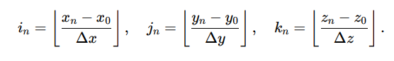
By the half-open voxel definition, membership is unique:

                                                                     p_n ∈ V_in,jn,kn .

Equivalently, the mapping: ε → {0,…,N_x − 1} × {0,…,N_y − 1} × {0,…, N_z − 1} sends each en to exactly one (i, j, k).

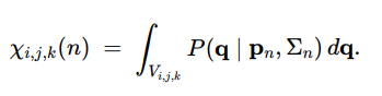
Probabilistic Assignment with Uncertainty Kernels

When an element has non-negligible footprint or uncertainty Σ_n, its presence may straddle voxel boundaries.

Let P (q| p_n , Σ_n) be the normalized spatial kernel induced by Σ_n around p_n.

Define the occupancy weight of element n in voxel (i, j, k) as

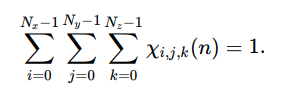
This satisfies:

– Range: 0 ≤ χ_i,j,k (n) ≤ 1 for all ( i, j, k).

– Partition of unity:

– Deterministic limit: if Σ_n → 0 and p_n lies strictly inside a single voxel, then

A common anisotropic Gaussian choice is

Occupancy Based Counts and Conservation

Define voxel counts by summing occupancies across elements:

Global conservation holds in both deterministic and probabilistic cases:

Thus, deterministic assignment yields one-hot membership , while probabilistic assignment yields soft membership that respects uncertainty and footprint overlap, both consistent with total element conservation.

Triple Sigma Occupancy

Let’s go over triple-sigma occupancy for one gaussian vossel. Let the voxel grid have unit cells and origin at (0, 0, 0). Consider a single Vossel en whose spatial kernel is an axis-aligned 3D Gaussian with mean near a voxel corner so that mass spills into neighbors:

– Mean (spatial center): μ = (μ_x, μ_y, μ_z) = (0.45, 0.45, 0.45)

– Standard deviations: σx = σ_y = σ_z = σ = 0.30

– Kernel: K(q) = N (q | μ, diag(σ², σ², σ²))

A voxel is

           V_i,j,k = [i, i + 1) × [j, j + 1) × [k, k + 1).

The probabilistic occupancy of this Vossel in V_i,j,k is

Because the kernel is separable (diagonal covariance), this factorizes into 1D Gaussian CDF differences along each axis:

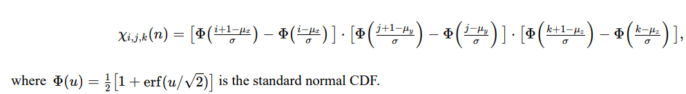
1D Slice Weights (shared for x, y, z)

With μ = 0.45 and σ = 0.30,

<img src=" https://www.opastpublishers.com/scholarly-images/9912-691e9d48b5e7d-a-unified-isr-world-model-vossels-voxels-mipvols-and-reinfor.png" width="400" height="100">

Numerically (with √2σ ≈ 0.424)

                                             w[−1,0) ≈ 0.0689, w[0,1) ≈ 0.8980, w[1,2) ≈ 0.0330,

 which sum to ≈ 1.000 per axis.

3D Voxel Occupancies (Top Contributors)

Since χ_i,j,k (n) is the product of the three 1D weights for the corresponding x, y, z intervals, the largest masses occur near the mean voxel [0, 1)³.

– Center voxel (i, j, k) = (0, 0, 0):

                                                χ0,0,0 = w³_0.1 ≈ 0.898³ ≈ 0.725.

– Face neighbors (one axis in neighbor cell), e.g. (1, 0, 0), (0, 1, 0), (0, 0, 1):

                                                    χ1,0,0 ≈ w[1,2)w2 ≈ 0.0266,

while negative-side faces (−1, 0, 0), (0,−1, 0), (0, 0,−1) give

                                                     χ−1,0,0 ≈ w[_−1,0)w_²0.1 ≈ 0.0555. 

– Edge neighbors (two axes in neighbor cells), e.g

                                           χ1,1,0 ≈ w2 w[0,1) ≈ 0.0010, χ1,−1,0 ≈ w[1,2)w[_−1,0)w[_0,1) ≈ 0.0020.

– Corner neighbors (three axes in neighbor cells):

                                           χ1,1,1 ≈ w³_1.2 ≈ 3.6 × 10⁻⁵, χ−1,−1,−1 ≈ w3^-1.0 ≈ 3.3 × 10^−4.

Compact Occupancy Table (approximate)

Voxel (i, j, k)	χi,j,k (n)
(0,0,0)	0.725
(-1,0,0), (0,-1,0), (0,0,-1)	0.0555 each
(1,0,0), (0,1,0), (0,0,1)	0.0266 each
(1,1,0), (1,0,1), (0,1,1)	0.0010 each
(1,-1,0) and perms	0.0020 each
(-1,-1,0) and perms	0.0043 each
(1,1,1)	3.6 × 10−5
(-1,-1,-1)	3.3 × 10−4

 

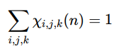
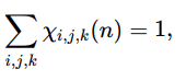
The sum over all voxels equals (within rounding) 1.0 because the kernel is normalized:

∑ χ_i,j,k(n) = 1.

i,j,k

Triple Sigma Truncation

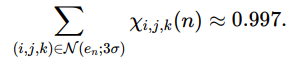
Because a 3D Gaussian concentrates ≈ 99.7% of its mass within 3σ along each axis, occupancy can be truncated to voxels within ±3σ of μ:

                               N (en; 3σ) = {(i, j, k) : [i, i + 1) ∩ [μx − 3σ, μx + 3σ] f= ∅, and similarly for y, z}.

Then

                                                 ∑                  χ_i,j,k(n) ≈ 0.997.

                                          (i,j,k)∈N (e_n;3σ) 

Takeaways

- Separable kernels reduce 3D occupancy integrals to products of 1D CDF differences.

- Most mass stays in the home voxel and face neighbors; edges and corners carry small tails.

- Triple-sigma truncation provides efficient computation with negligible loss.

- These χ_i,j,k (n) feed directly into voxel counts, weighted aggregates, and kriging/co-kriging estimators.

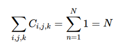
Global Conservation Identity

The voxel counts are defined as aggregated occupancies:

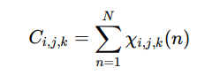
where χ_i,j,k (n) is the occupancy weight of element en in voxel V_i,j,k .

Step 1: Total Count Over Grid

Summing across all voxels in the grid gives

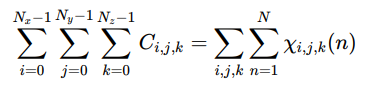
Step 2: Exchange the Order of Summation

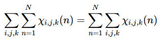
By linearity, the order of summation can be swapped

Step 3: Deterministic Case

If each element e_n lies fully inside a single voxel (hard assignment), then

since exactly one voxel receives membership χ_i,j,k (n) = 1 and all others receive 0.

Therefore,

Step 4 :Probabilistic Case

If elements are modeled with uncertainty kernels Σ_n, then occupancies are fractional but normalized:

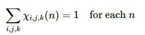
because χ_i,j,k (n) partitions the unit mass of the distribution P (q â?£ p_n, Σ_n) across the voxel grid.

Hence

Interpretation

This identity shows that the voxelized representation is conservative: the total count of elements is invariant under discretization.

Whether occupancy is hard (one-hot) or soft (fractional), the sum over all voxels always recovers exactly the total number of elements N.

Triple Sigma Interpretation

When the uncertainty kernel Σ_n is modeled as a Gaussian covariance, the occupancy weights χ_i,j,k (n) are defined as integrals of the Gaussian probability density over each voxel V_i,j,k:

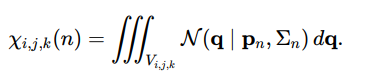
Step 1: Gaussian Mass Concentration

For a univariate Gaussian distribution, approximately 99.7% of the probability mass lies within ±3σ of the mean. In three dimensions, the joint kernel is separable along principal axes, so nearly all of the probability is concentrated inside the cube:

Step 2: Restricting the Neighborhood

Define the triple-sigma neighborhood of element en as the set of voxels whose support overlaps this region:

Step 3: Conservation Within Triple-Sigma

By construction, the sum of occupancies restricted to this neighborhood captures nearly all of the Vossel’s probability mass:

The small remainder outside this region corresponds to the Gaussian tails, which can be safely neglected for most ISR applications.

Step 4: Practical Implication

This triple-sigma truncation provides a principled cutoff for voxel assignment in probabilistic mode. It ensures:

– Computational tractability by limiting the number of voxels evaluated per element.

– Statistical fidelity by preserving almost all of the probability mass.

– Consistency with Gaussian probability bounds, giving an interpretable error margin.

In effect, each Vossel’s probabilistic spread can be localized to a finite set of voxels without losing more than 0.3% of the probability mass. This guarantees both efficiency and fidelity in voxelized aggregation, kriging, and reinforcement learning workflows.

Set Containment

A voxel grid partitions the spatial domain D ⊆  into disjoint cells {V _i,j,k}.

Each Vossel en has a nominal center p_n = (x_n, y_n, z_n). 

To ensure well-defined indexing, every element must fall inside the support of the grid.

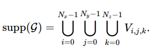
Step 1: Grid Support

The union of all voxels defines the domain covered by the grid:

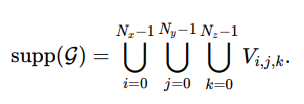
This is the finite region of space where voxelization is valid.

Step 2: Containment Requirement

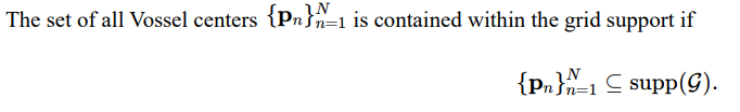
That is, every element lies in at least one voxel. 

Step 3: Element-to-Voxel Existence

Equivalently, this requirement can be stated in elementwise form:

                                                                ∀n ∈ {1, … , N }, ∃(i, j, k) such that p_n ∈ V_i,j,k.

This guarantees that each Vossel has a unique voxel assignment under the half-open voxel boundary convention.

Step 4: Boundary Handling

Because voxel intervals are half-open (closed on the lower bound, open on the upper), boundary cases are uniquely assigned.

For example, a point at x = x₀ + (i + 1)Δx belongs to voxel V_i+1,j,k, not V_i,j,k, avoiding ambiguity at shared faces.

Step 5: Probabilistic Occupancy Case

When Vossels carry uncertainty kernels Σ_n, set containment extends to distributional support.

Instead of a single voxel, the kernel spreads mass across neighbors:

so that total membership is still contained within the grid, even if distributed probabilistically.

Set containment enforces that all Vossels are represented within the voxelized domain.

Deterministically, each point belongs to exactly one voxel; probabilistically, occupancy spreads across multiple voxels but remains normalized to the grid support.

This property guarantees global conservation of mass and ensures that subsequent aggregation, interpolation, and fusion remain well- posed.

Aggregation Over Voxels

Once Vossels are assigned to voxels, we can aggregate per-element quantities into voxel-level summaries.

This provides a bridge from atomic measurements to gridded statistics while preserving conservation.

Step 1: Per-Element Function

Let f : ε →  be any scalar-valued function defined on the element set.

Examples include:

– f (e_n) = intensity or amplitude,

– f (e_n) = confidence score,

– f (e_n) = indicator of a material class.

Step 2: Voxel-Wise Aggregation

For voxel (i, j, k), define the aggregated statistic:

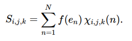
Here χ_i,j,k (n) is the occupancy of element e_n in voxel V_i,j,k, which equals 1 if deterministic membership holds, or a fractional weight in the probabilistic case.

Step 3: Deterministic Case

If χ_i,j,k (n) ∈ {0, 1} , then S_i,j,k is simply the sum of f (e_n) over all elements whose centers fall in voxel ( i, j, k).

Step 4: Probabilistic Case

If e_n spans multiple voxels, each voxel receives a fractional contribution:

Thus, S_i,j,k becomes a weighted contribution proportional to the overlap of the uncertainty kernel with the voxel.

Step 5: Global Conservation

Summing across all voxels yields:

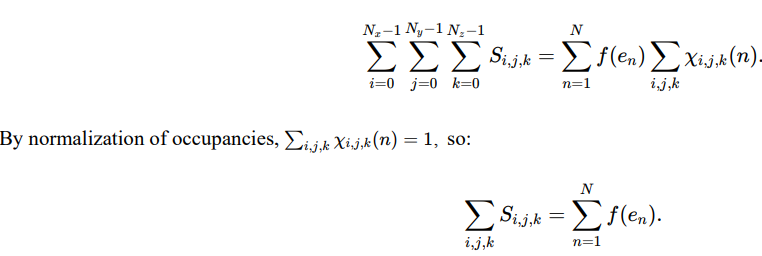
This states that the total aggregated value over the grid equals the total over all elements, guaranteeing no loss or duplication.

Step 6: Interpretation

– If f (e_n) = 1, then S_i,j,k counts elements, and conservation says the total count across voxels is N.

– If f (e_n) is intensity, then S_i,j,k represents voxel-level energy accumulation, conserved across the grid.

– If f (e_n) is a class indicator, then S_i,j,k is a soft histogram of class membership over space.

Aggregation over voxels generalizes counting to arbitrary per-element functions.

It supports deterministic or probabilistic assignments, while ensuring global conservation of sums.

This mechanism enables voxelized statistics such as densities, intensities, or class distributions, forming the basis for kriging, interpolation, and reinforcement learning rewards.

Multiresolution (MipVols)

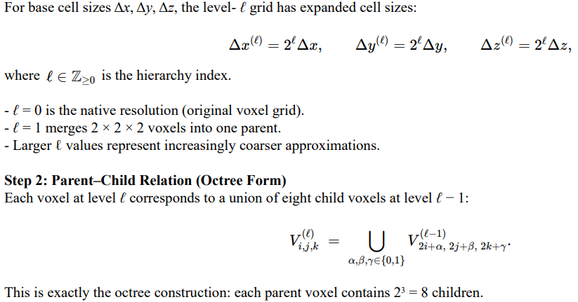
Thus, no matter how coarse the hierarchy, the total number of elements represented remains exactly N.

Step 5: Interpretation

– At = 0, each Vossel contributes at its native voxel.

– At  = 1, contributions are aggregated into 2 × 2 × 2 blocks, yielding a coarser but still conserved representation.

– At higher , the hierarchy provides a pyramid of representations, enabling algorithms to operate at appropriate levels of detail.

Step 6: Applications

– Visualization: low-resolution mipvols allow fast rendering of large datasets.

– Queries: hierarchical search reduces computation, as coarse queries prune regions before refinement.

– Learning: reinforcement learning agents can train on coarse levels first, then refine at fine levels (curriculum training).

– Storage: mipvols provide a natural compression hierarchy while retaining conservation guarantees.

The mipvol hierarchy organizes voxel grids into multiresolution levels with exact conservation of counts and attributes. This provides adaptive fidelity, computational efficiency, and scalability across CPUs, GPUs, and clusters, while ensuring that total measurements remain consistent across all levels.

Abstract Representation of a Vossel Sample

Unifying heterogeneous sensor feeds requires more than reducing each observation to a spatial point. Every measurement carries a finite region of influence dictated by sensor physics and projection geometry. This influence is represented in two layers. The first is the projected geometry, a deterministic approximation of the footprint imposed by the sensing system. The second is the statistical variance, which captures the uncertainty, blur, and distortion introduced by optics, propagation, and the environment.

Projected geometry provides a first-order mapping of how a measurement interacts with the world. LiDAR pulses expand as cones terminating in circular or elliptical patches on terrain. Optical pixels, under camera models, project to quadrilaterals on the ground corresponding to detector array positions. SAR resolution cells are oriented ellipses, defined by range resolution along one axis and azimuth along another. These geometric approximations enable disparate sensors to be aligned in a shared model. Importantly, Fr is not a hard boundary but an envelope of strongest influence. True sensitivity distributions extend beyond this region, overlapping adjacent measurements.

The physical response is always softer than geometry alone suggests. Optical pixels exhibit Gaussian-like point spread functions (PSFs), causing gradual roll-off and overlap between neighboring pixels. LiDAR returns carry beam spread and sub-sampling artifacts that extend influence beyond the ideal cone. Radar and acoustic samples smear anisotropically with incidence angle, terrain slope, and propagation medium. These effects cannot be reduced to geometry and require a probabilistic description.

For this reason, each measurement is paired with a statistical kernel Σ_r that models the distribution of influence around its nominal footprint. In isotropic cases, this may be a circular Gaussian centered on the projection. In anisotropic cases, it becomes an oriented ellipse stretched along sensor geometry or environmental gradients. Beyond Gaussians, certain sensors exhibit higher-order or multimodal kernels: optical Airy disks, radar speckle, or acoustic side lobes. Variance extends naturally to time (latency, timestamp jitter) and spectrum (wavelength calibration error, quantization), broadening the kernel concept beyond space alone.

The duality of projected geometry F_r and statistical variance Σ_r defines a generalized sensor model. The geometry encodes the deterministic footprint implied by the measurement system, while the variance describes the uncertainty cloud that softens this boundary. This abstraction makes LiDAR pulses, SAR cells, EO pixels, and acoustic lobes mathematically equivalent: volumetric elements with a footprint and a probability distribution. On this basis, one can construct unified operations for fusion, normalization, and multi-modal extraction across all sensing modalities.

Voxels and MipVols

The Vossel abstraction defines the atomic measurement, but voxels and their mipvol hierarchies provide the computational structure that makes the framework operational at scale. Each Vossel is assigned to a voxel grid, introducing spatial locality and enabling efficient neighborhood search. This binning step is essential, since direct querying of billions of raw samples across ISR datasets would be computationally prohibitive.

The mipvol hierarchy extends this organization into multiple resolutions. Fine-scale fidelity is preserved where the task requires detail, while coarser levels accelerate retrieval in regions where the projected target size does not demand native resolution. In this way, the hierarchy provides adaptive fidelity, balancing precision against computational load.

Although a Vossel is independently defined, voxel and mipvol layers form the scaffolding required for tractable implementation. They ensure scalability, efficient retrieval, and manageable memory use, making the representation viable for enterprise-level ISR exploitation.

Formalization

Each sensor reading r is represented as a Vossel sample V_r, which has two components:

1. Projected Geometry (Footprint) – the first-order geometric envelope of the region covered by the measurement.

2. Statistical Variance (Uncertainty Kernel) – the second-order stochastic representation of positional error, blur, and distortion.

Projected Geometry

Let p = (x, y, z) be the nominal measurement location.

Define the footprint shape F_r as the envelope in space where the sample is expected to have influence.

This footprint is never truly bounded by sharp edges; instead, it is modeled as an idealized form that represents the primary extent of the sample, while acknowledging that the physical sensitivity function has gradual roll-off and overlap with adjacent samples.

Examples:

- LiDAR: F_r is modeled as a cone truncated at terrain with radius set by beam divergence. In reality, the beam has a Gaussian profile, producing a soft-edged circular patch with energy spread beyond the nominal radius. LiDAR beam divergence, unlike EO/IR, is narrower than sampling distance, leading to unavoidable subsampling artifacts.

- EO/IR Pixel: F_r is modeled as a quadrilateral (or ellipse) projected onto terrain from camera geometry. Physically, the pixel integrates light according to the optical point spread function (PSF), leading to Gaussian-like roll-off and overlap between adjacent pixels.

- SAR Resolution Cell: F_r is modeled as an oriented ellipse defined by range and azimuth resolution. The actual response includes sidelobes and speckle, which smear energy outside the ideal ellipse.

- Acoustic/ELINT Sample: Fr is modeled as a lobe or sector volume derived from beam pattern. True reception patterns often have side lobes and irregularities that extend sensitivity beyond the modeled volume.

Formally, the footprint can be described as:

                                                                    F_r = T_r(Ω₀)

where Ω₀ is a canonical shape (circle, ellipse, quadrilateral, cube) and T_r is the sensor-specific transform (projection, warping, terrain interaction, atmospheric distortion).

The statistical variance term Σ_r then augments F_r by encoding the blurred, probabilistic distribution of energy around and beyond this idealized footprint.

Statistical Variance (Sphere of Confusion)

Each footprint² is associated with an uncertainty kernel Σ_r , typically a covariance matrix in , though it may be extended to to also capture temporal uncertainty as well.

– Isotropic noise: Σ_r = σ² I → spherical circle of confusion.

– Anisotropic distortion: Σ_r elliptical, stretched along terrain slope or projection angle.

– Atmospheric or propagation spread: elongation of Σ_r along line-of-sight.

– Spectral or radiometric variance: additional components can be modeled for calibration error or noise in {λ_i} or {a_j}.

The probability density of the true measurement location q is:

<img src=" https://www.opastpublishers.com/scholarly-images/9912-691eb6537a7db-a-unified-isr-world-model-vossels-voxels-mipvols-and-reinfor.png" width="400" height="100">

Composite Representation

A Vossel sample V_r is then defined as:

                                            V_r = (p, Fr, Σr, {λ_i}, {aj })

Where:

– p = (x, y, z, t): nominal center

– F_r: projected geometry (footprint envelope)

– Σ_r : statistical variance kernel (uncertainty/confusion)

– {λ_i }: spectral/temporal attributes³

– {a_j}: sensor-specific metadata (intensity, phase, Doppler, etc.)

Interpretation

– Projected Geometry = how the sensor paints the world (physical footprint).

– Statistical Variance = confidence in the placement of that footprint in space, extended if needed into time and spectral dimensions^4,5.

– Together they define a probabilistic volumetric element (a Vossel) with both extent and noise.

– This abstraction allows heterogeneous sensors to be integrated consistently, with uncertainty explicitly represented in the same mathematical (and computer data structure) framework.

Full Form

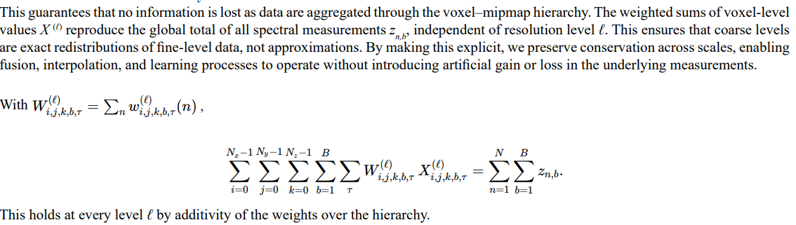
Let’s take the Vossel element data and combine it with voxel coherency to get our expanded voxel-band-time process:

For resolution level , voxel (_{i, j, k}), spectral band b, and time bin τ , define

<img src=" https://www.opastpublishers.com/scholarly-images/9912-691eb96b3d9cc-a-unified-isr-world-model-vossels-voxels-mipvols-and-reinfor.png" width="300" height="100">

And expand our notation to clarify implementation and show how spatial, temporal, and spectral weights arise from integrals over kernels and regions and eliminating any confusion over what χ, θ, η mean. As such, let’s put into the expanded form:

<img src=" https://www.opastpublishers.com/scholarly-images/9912-691eb9c290e14-a-unified-isr-world-model-vossels-voxels-mipvols-and-reinfor.png" width="400" height="100">

This traverses all voxels, bands, and time bins, and for each, sums over all elements with weights that incorporate spatial occupancy, temporal occupancy, spectral mixing, and mipmap additivity. The numerator aggregates all element contributions; the denominator normalizes by total occupancy weight.

Mipmap Consistency in the Weights

This ensures that aggregation across levels is mathematically consistent. The spatial occupancy χ is additive over its eight children in the octree, and the full weight w, when combined with temporal and spectral terms, inherits the same child→parent recursion. This means that parent voxels represent the exact sum of their children, not an approximation. By making this explicit, we guarantee that queries and fusion operations remain conservative across resolutions, and rein-forcement learning agents can transition between coarse and fine levels without losing consistency or violating conservation laws. Spatial occupancy is additive across the octree:

 

Therefore the full weight

<img src=" https://www.opastpublishers.com/scholarly-images/9912-691ebb693f035-a-unified-isr-world-model-vossels-voxels-mipvols-and-reinfor.png" width="500" height="100">

inherits the same child→parent recursion

<img src=" https://www.opastpublishers.com/scholarly-images/9912-691ebb96a4e1e-a-unified-isr-world-model-vossels-voxels-mipvols-and-reinfor.png" width="500" height="100">

Spectral Mixing

R_b (λ) is the bandpass (spectral response) of band b. μn is the element’s spectral measure. The mixing coefficient is

<img src=" https://www.opastpublishers.com/scholarly-images/9912-691ebe281eeb1-a-unified-isr-world-model-vossels-voxels-mipvols-and-reinfor.png" width="300" height="100">

For band-isolated _znb,set η_b (n) = 1

Global Conservation Identity

Supporting Definitions

Spatial kernel (projected geometry + uncertainty) 

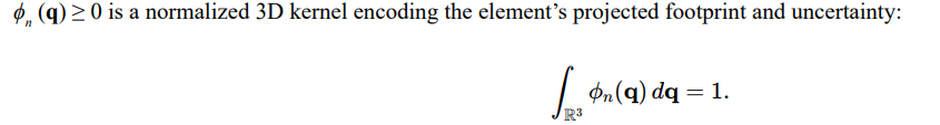
Typical construction: pushforward of a canonical PSF through the sensor projection and terrain/medium mapping, with anisotropy governed by Σ_n.

Temporal Kernel

ψ_n (t) ≥ 0 is a normalized 1D kernel for acquisition time and its uncertainty:

Selection Mask

1_Ω (q) ∈ {0, 1} restricts to regions of interest (e.g., the view frustum). Omit or set to 1 for full-domain accumulation.

Variable and Index Recap

Elements and measurements

e_n: the n-th Vossel (element).

p_{n =} (xn, yn, zn, tn): nominal center of e_n.

F_n: projected footprint envelope of e_n.

Σ_n: uncertainty kernel parameters for e_n.

z_n,b: scalar value of en in band b (radiance, intensity, etc.).

μn (λ): spectral measure of en (discrete spectrum or density).

Spatial grid and hierarchy

<img src=" https://www.opastpublishers.com/scholarly-images/9912-691ec12e8fc57-a-unified-isr-world-model-vossels-voxels-mipvols-and-reinfor.png" width="500" height="600">

special cases

Deterministic point elements

 

Sensors Considered

The sensors listed demonstrate the flexibility of the Vossel abstraction. A single atomic representation can cover imaging, radar, LiDAR, acoustic, seismic, magnetic, gravimetric, environmental, cyber, and jamming sources. Vossels are important because they preserve geometry and uncertainty while unifying different observables into one structure. All sensor feeds can be kept in one place and rep- resented at their native resolution, even though the modalities vary widely in scale and character. This creates a centralized repository that allows radically different data types to coexist and be fused within a consistent world model.

 

 

Terahertz Imaging	0.3–10 THz imagers	Radiance, spectral features	As EO	Attenuation, multipath	Near-field footprints; short range
Terrestrial LiDAR (TLS)	Tripod, polar scan	Range, reflectance	Polar sampling geometry	Occlusion, registration	Very high density; station metadata
Thermal ISR (MWIR/LWIR)	Airborne pods, ground imagers	Radiance / brightness temp	As EO	Emissivity, atmos attenuation	Add σ_T; calibration drift attributes
Through-wall Radar	UWB imaging	Range profiles	Wall-aligned ellipses	Multipath	Ellipsoids behind walls; building model attributes
Tomographic SAR (TomoSAR)	Multi-baseline stacks	3D reflectivity volumes	Elliptical stacks	Vertical resolution limits	Bands per altitude bin; sparsity priors
UWB Localization	Impulse radio, RF ranging	Ranging/TDOA	Spheres/shells	Clock sync	Iso-range shells; multi-node intersection
WAMI (Wide Area Motion Imagery)	Persistent EO	Coarse pixels, high frame rate	Large projected quads	Registration error	Tight temporal bins; motion emphasis
Wi-Fi/5G Sensing	CSI, device-free localization	Range/angle changes	Volumetric near nodes	Multipath	Small lobes; anomalies mapped as Vossels

Clarifications

Clarifications are necessary since the terminology employed here overlaps with conventional computer graphics. Voxels may either hold data values directly or serve as spatial organizers with pointers. In medical imaging, voxels typically contain measured values, whereas in ray tracing they are used to spatially organize geometry for rapid culling. Confusion arises when both interpretations are used interchangeably. Another challenge of voxel-based processing is adaptive resolution, often referred to as the “teapot in the stadium problem.” Vossels address this issue through mipvols, which provide scalable multiresolution structures. It should also be noted that voxels are not restricted to Cartesian space; they may occupy spherical, Fourier, or octahedral domains, among others. Recent work by Chan and Haldar demonstrates the use of voxels in k-space for medical imaging, a trend that applies here as well [9]. Vossels can be extended into temporary or permanent alternate domains as required, maintaining consistency of representation across coordinate systems.

Ongoing Work

Current work is focusing on the detailed mechanics of Vossel implementation. The mathematical and structural framework established here is being extended into full integration processes. Efforts are underway to construct voxel hierarchies from raw sensor feeds, including projection, kernel integration, uncertainty propagation, and occupancy weighting. Retrieval procedures are being demonstrated, showing how spatio–temporal–spectral queries are resolved using direct kriging, hybrid voxel–kriging, and mipmap-based approximations.

Research is also addressing ingestion of ISR modalities—ELINT, EO/IR, SAR, LiDAR, acoustic, seismic, environmental, cyber, and jamming—into the Vossel model. This includes transforms from native data formats to Vossel-compatible representations, with emphasis on preserving geometry, uncertainty, and spectral content. Localized spherical voxel spaces are more attuned to sensor polar resolu- tions, and for simulation, Plücker Space is convenient in ray intersection tests [10]. In parallel, the design is being developed with an eye toward hardware acceleration, particularly through FPGA-based prototypes and potential ASIC implementations. Embedding Vossel ingestion and fusion directly into hardware reduces the computational resources required, making it feasible for in-field edge use where size, weight, and power constraints limit conventional processing.

System-level integration is also being advanced, including view-frustum extraction pipelines for interactive visualization, distributed storage for large ISR data streams, and optimization of mipmap consistency across networked systems. The aim is to make the Vossel framework directly usable in ISR fusion engines, simulation environments, and operational planning tools.

These activities are moving the emphasis from theoretical formulation to reproducible implementation, establishing precise algorithms, benchmarks, and hardware pathways so that Vossel-based fusion can be deployed and evaluated in live ISR environments.

References

1. Cerdeira-Pena, A., de Bernardo, G., Fariña, A., Paramá, J. R., & Silva-Coira, F. (2018, September). Towards a compact representation of temporal rasters. In International Symposium on String Processing and Information Retrieval (pp. 117-130). Cham: Springer International Publishing.
2. Abdelguerfi, M., Givaudan, J., Shaw, K., & Ladner, R. (2002, November). The 2-3TR-tree, a trajectory-oriented index structure for fully evolving valid-time spatio-temporal datasets. In Proceedings of the 10th ACM international symposium on Advances in geographic information systems (pp. 29-34).
3. Forlizzi, L., Güting, R. H., Nardelli, E., & Schneider, M. (2000). A data model and data structures for moving objects databases.ACM SIGMOD Record, 29(2), 319-330.
4. Nishida, S., Saiwaki, N., & Naka, A. (2002, November). An adaptive spatio-temporal data management structure for efficient search. In Proceedings 6th IEEE International Workshop on Robot and Human Communication. RO-MAN'97 SENDAI. IEEE.
5. Reddy, S., Kothapalli, A., Varshini, K. S. S., Nandhan, R., & KV, V. (2024, November). Space Debris Clustering and Avoidance Using Chrono-Spatial Computational Frameworks. In 2024 International Conference on Intelligent Computing and Emerging Communication Technologies (ICEC) (pp. 1-6). IEEE.
6. Wang, Y., Hijikata, Y., & Nishida, S. (2003, March). A study on a spatio-temporal data structure for managing video data from monitoring cameras. In 17th International Conference on Advanced Information Networking and Applications, 2003. AINA 2003. (pp. 454-461). IEEE.
7. Zhang Lifu, Chen Hao, Sun Xuejian, Fu Dongjie, & Tong Qingxi. (2017). Design of integrated storage structure for multi- dimensional remote sensing data in terms of space, time and spectrum. Journal of Remote Sensing, 21(1).
8. Samet, H. (2006). Foundations of multidimensional and metric data structures. Morgan Kaufmann.
9. Chan, C. C., & Haldar, J. P. (2025). A New k-Space Model for Non-Cartesian Fourier Imaging. arXiv preprint arXiv:2505.05647.
10. Marmitt, G., & Slusallek, P. (2005). Fast ray traversal of unstructured volume data using plucker tests. Computer Graphics Lab, Saarland University. Technical report.