A Taxonomy of Solutions for Fixed-Radix FFT Algorithm

Introduction

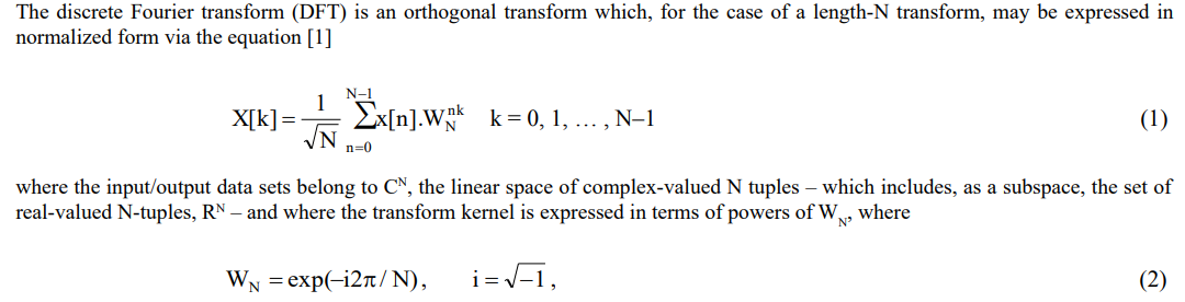
the primitive Nth complex root of unity [2,3] – the normalizing term 1 N will be left out of equations hereafter for ease of analysis. Fast solutions to the DFT are based upon the divide and conquer principle and referred to generically as fast Fourier transform (FFT) algorithms [5,6,13]. When the transform length N is expressible as some power of a fixed arbitrary positive integer, R, such that

N=R^{s                                                                                             (3)}

for some integer s > 1, the algorithm is referred to as a fixed-radix FFT with radix R (or, more simply, as a radix-R FFT) and possesses the attraction that the associated arithmetic complexity, relative to that resulting from the direct computation of the DFT, may be reduced from O(N 2 ) to just (N× log N) arithmetic operations, this being achieved through the exploitation of those trigonometric symmetries present in the DFT definition. Much of the existing technical literature on the fixed-radix FFT algorithm deals with those simple cases where the radix takes on a value of either two or four, whereas this paper, which is of a tutorial nature, generalizes the results so as to cater for the generic case where the radix R can take on any positive integer value.

The complex-valued exponential terms, Wn_Nk , as derived from the primitive Nth complex root of unity of Equation 2, each comprise two trigonometric components, one sinusoidal and the other cosinusoidal, with each pair being more commonly referred to as twiddle factors [5,13]. These are required to be fed, R at a time, to the computational unit used for carrying out the FFT algorithm’s repetitive arithmetic operations which, for a radix-R transform, is denoted herein by CUR (where the subscript ‘R’ refers to the radix) and involves the production of R complex-valued outputs from the multiplicative combining, in an appropriate fashion, of the R twiddle factors with R complex-valued (or real-valued) inputs.

The radix-R version of the fixed-radix FFT is a recursive algorithm that’s obtained from the breaking down or decomposing of the original problem of the length-N transform – and, in similar fashion, of each of the resulting sub-problems – into R smaller sub-problems each with size being subsequently reduced by a factor of 1/R. The end result of such a decomposition is the conversion of the original problem, namely that of a single length-N transform, into logRN computational stages, where each stage comprises N/R independent CUR’s and where the execution of a given stage can only commence once that of its predecessor has been completed, so that the FFT output is produced on completion of the final computational stage. Thus, the recursive decomposition of the original length-N transform results in a total of

identical sub-problems, where each sub-problem corresponds to that of a single CUR. As a result of this algorithmic regularity – which equates to the amount of repetition and symmetry present in the design – the design complexity of the radix-R FFT reduces to that of a single CUR, whilst the associated arithmetic complexity of the radix-R FFT is, in turn, directly dependent upon that of the CU_R.

There are various ways in which such a decomposition of the fixed-radix FFT might be achieved and a task of this paper is to describe the main options in order to provide the algorithm designer with the information needed to make informed decisions when looking to implement such an algorithm in an efficient manner that’s best able to exploit the available computing equipment, whether geared to sequential (single processor) or parallel (multiple processor) computation. This involves describing: 1) the two decimation scheme variants used for breaking down the original problem of the length-N radix-R transform (and of each of the resulting sub-problems) into R smaller sub-problems, one variant of which is carried out in the time domain, being referred to as the decimation-in-time (DIT) approach, and the other in the frequency domain, being similarly referred to as the decimation-in-frequency (DIF) approach; and 2) the index mappings – namely the lexicographic or naturally-ordered (NAT) and digit reversal (DR) mappings – arising from such a decomposition and at what stage of the computation they might each be applied [5,13].

Thus, following this introductory section, the paper continues in Section 2 with descriptions of the CUR required by the radix-R FFT together with the types of decimation scheme and the associated index mappings. It is then seen in Section 3 how these various techniques might be appropriately combined to yield the four most commonly used algorithmic variations of the radix-R FFT, with a more detailed discussion given in Section 4 of the various schemes available for the efficient generation of the twiddle factors including the associated trade-off of arithmetic complexity against memory requirement. A brief account is then provided in Section 5 of those techniques – as defined over both spatial and temporal domains – that might be exploited in order to facilitate the efficient parallel computation [4] of the radix-R FFT when suitably defined parallel equipment is available for its implementation. The paper concludes in Section 6 with a brief summary and conclusions.

Basic Structure of Fixed-Radix FFT Algorithm

The recursive structure of the radix-R version of the fixed-radix FFT is perfectly illustrated in Figure 1, where the central role played by the CUR in the transform’s recursive computation is apparent. After a brief description of this key component the index mappings required for the reordering of the data are described together with the two types of decimation scheme required for the decomposition of the original length-N transform (and of each of each of the resulting sub-problems) into R smaller sub-problems, each with size being subsequently reduced by a factor of 1/R, leading eventually to logRN stages, each of N/R independent CUR’s which may each be easily solved.

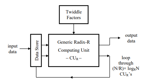
Figure 1: Sequential Processing Architecture for Length-N Radix-R FFT

The Computational Unit

The key component of the radix-R FFT is that of the computational unit, CUR, which executes the small sub-problems arising from the transform’s recursive decomposition. For the most commonly adopted radices, namely those with values of two or four, the unit is more commonly known as the butterfly or dragonfly, respectively, this naming being due to the fact that the data within the resulting computational structure flows in a pattern that resembles that of the wings of the corresponding insect, respectively [5,13]. Note that, technically, an insect with many wings, as is relevant here for the radix-R transform, might be referred to as a polyptera (meaning many wings) or possibly a polyfly, so that our computational unit, CUR, might well be referred to as such for consistency with the previous two wing and four-wing definitions. Perhaps its best, however, not to get too entomological in a paper like this as most engineers will tend to use the word ‘butterfly’ regardless of the size or shape of the computational unit. A detailed description of CUR, in terms of its signal flow graph (SFG), is clearly dependent upon the choice of decimation scheme and the placement of the corresponding index mappings and is therefore best discussed in the relevant descriptions provided in Section 3 where the four main algorithmic variations of the fixed-radix FFT are to be addressed.

Data Reordering Mappings – Digit-Reversal and Natural Ordering

The data reordering required by the fixed-radix FFT involves both the NAT (which simply leaves the data addresses in their original unscrambled or lexicographic form) and DR mappings, where for a radix-R FFT the DR mapping simply reverses the base-R digits of the data addresses. The relevance of the DR mapping is due to the fact that the overall effect of the radix-R FFT is to produce an output data set where the data addresses are permuted or scrambled, relative to those of the input data set, according to the DR mapping. Thus, if the input data set is ordered according to the NAT mapping then the output data set will be ordered according to the DR mapping, whilst if the input data set is ordered according to the DR mapping then the output data set will be ordered according to the NAT mapping (given that the DR mapping is its own inverse so that applying it twice reduces to that of the identity mapping). For the case of the radix-2 FFT, the DR mapping reduces to the familiar bit-reversal (BR) mapping, which simply reverses the data addresses, one bit at a time, whilst for the radix-4 FFT, the DR mapping reduces to the di-bit reversal (DBR) mapping, which reverses the data addresses, two bits at a time [5,13]. Thus, when the radix R is expressible as a power of two, the digit reversal is quite straightforward, as each digit consists of an exact integer number of bits, namely log2R, enabling the data addresses to be reversed log2R bits at a time. When this is not the case, however, then each of the data addresses needs to be represented by means of an appropriate m-ary number, such as (d4,d3,d2,d1,d0) for the case of the radix-5 FFT, which upon reversal is given by (d0,d1,d2,d3,d4), with the most/least significant bit thus becoming the least/ most significant bit.

Decimation Schemes – Time-Domain and Frequency-Domain

The first decimation scheme to be discussed is that of the DIT which, for the simple case of the radix-2 FFT (illustrated here for ease of analysis), involves the splitting up of the time-domain input data set into two interleaved (and thus independent) subsets: those input samples with even-numbered addresses and those with odd-numbered addresses – noting that extending this to the radix-4 algorithm involves splitting the even-numbered addresses into two interleaved subsequences of even-numbered addresses and the odd-numbered addresses into two interleaved subsequences of odd-numbered addresses, and so on for higher power-of-two radices. For the case of the length-N transform, the two interleaved subsets, each of N/2 input data samples, are then processed separately with the first stage of the recursion being solved by putting

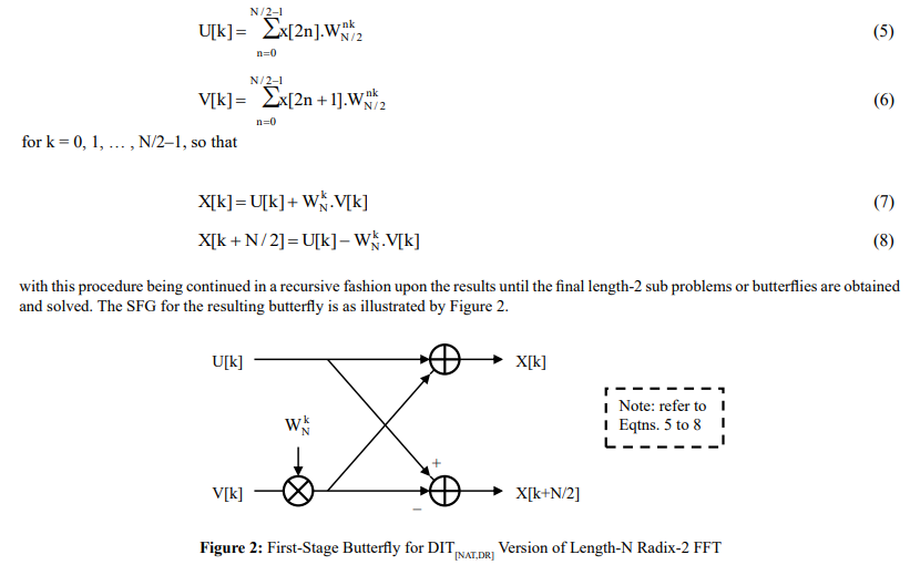
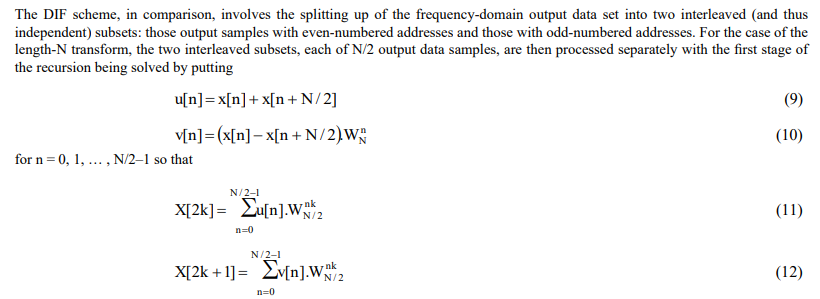
for k = 0, 1, … , N/2–1, with this procedure being continued in a recursive fashion upon the results until the final length-2 sub-problems or butterflies are obtained and solved. The SFG for the resulting butterfly is as illustrated by Figure 3.

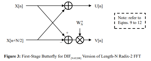
Note, that with both decimation schemes, for the case of a radix-2 FFT, each pair of outputs is produced from those inputs possessing the same pair of addresses such that the inputs do not enter into the computation of any other pair of outputs. Since the computation for this two-fold input/output data set (which is commonly referred to in the literature as a dual node) is independent of all others, the computation may be carried out in an in-place fashion whereby the outputs simply overwrite the inputs in memory. Also, the addresses of the inputs for any given two-fold independent output data set are separated by an amount that is fixed for the particular stage of butterflies that are being carried out, this distance between addresses being referred to as the stride. Clearly, the stride will be different for each stage of butterflies, as will be discussed in greater depth in Section 3. Finally, the concept of the two-fold input/ output data set generalizes in an obvious fashion to the case of the radix-R FFT whereby the relevant data set is split into R interleaved subsets and where each R-fold output data set is produced from those inputs possessing the same set of R addresses, in an in-place fashion, such that the inputs do not enter into the computation of any other R-fold output data sets.

Discussion

Whichever of the above two decimation schemes is used, the result is that the computation of the length-N radix-2 FFT is reduced to the computation of a number of butterflies (as given by Equation 4 with the value of ‘R’ being set to two), which are easily solved, with extension to the radix-R case reducing in similar fashion to the computation of a corresponding number of independent CUR’s. There can be some confusion in the existing technical literature whereby it is often assumed that the input data set to the DIT version of the fixed radix FFT needs to be ordered according to the DR mapping and the output data set according to the NAT mapping and that, similarly, for the DIF version of the fixed radix FFT, the input data set needs to be ordered according to the NAT mapping and the output data set according to the DR mapping. This is not the case, however, as the input/output data set for either decimation scheme may be ordered according to either index mapping, as will be discussed in Section 3. An additional option (although not one considered here) involves having both the input and output data sets ordered according to the NAT mapping, but this approach – referred to as an ordered FFT [5,15] which may be based upon either DIT or DIF versions of the fixed-radix FFT – involves the introduction of additional complexity through having to reorder the data and the twiddle factors between the radix-R FFT’s multiple stages of independent CU_R’s.

Algorithmic Variations for Fixed-Radix FFT Algorithm

As already stated, much of the existing technical literature on the fixed-radix FFT deals with only two variations for the simple radix-2 and radix-4 cases: the DIT scheme with DR ordered input data and the DIF scheme with DR ordered output data, which clearly provides one with a limited account of the available options. To address this situation, four algorithmic variations are discussed in this section for dealing with the generic radix-R version of the fixed-radix FFT, these being distinguished from one another by the choice of decimation scheme and the placement of the index mappings. For the radix-R transform, these particular choices determine: 1) the stride, relating to the stage dependent address spacing of the R-fold interleaved input data sets to the CU_R, which will differ from one stage of independent CU_R’s to the next, as well as 2) the number and size of distinct sets of independent CU_R’s, per stage, where each set requires its own distinct set of R twiddle factors. Each variation is illustrated here by means of a simple length-4 radix-2 FFT which comprises just two stages, with each stage involving the computation of two CU₂’s or butterflies – note that for each of the illustrations provided in this section, wherever an input to an adder has no sign attached, a plus sign is to be assumed.

The DIT Algorithm with Scrambled Output Data

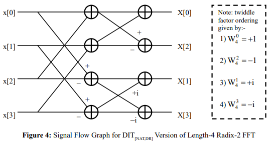
The DIT version of the radix-R FFT, where the input data set is ordered according to the NAT mapping and the output data set according to the DR mapping, is denoted hereafter by DIT_[NAT,DR] – see the example of Figure 4 where, from the SFG, it is evident that the powers of W4 must be ordered according to that of the output data set, namely via the BR mapping. The stride for the first stage of butterflies has a value of two, whilst the stride for the second stage of butterflies has a value of one. Generalizing, for the case of a length-N radix-R FFT, the stride will decrease from one stage to the next by means of a multiplicative scale factor of 1/R, with the first stage having a value of N/R and the last stage having a value of one and the twiddle factors ordered according to that of the output data set, namely via the DR mapping. Also, the first stage involves just one set of N/R independent CU_R’s, all using the same set of R twiddle factors, whilst the second stage involves R sets, each of N/R2 independent CU ’s, with those CU ’s in each set using the same set of R twiddle factors. R R Continuing in this fashion, with the number of CU_R sets increasing from one stage to the next by a multiplicative scale factor of R, it is evident that the last stage involves N/R sets, each of just one CU_R, with that CU_R using its own distinct set of R twiddle factors (so that the last stage exploits all N twiddle factors).

The DIT Algorithm with Scrambled Input Data

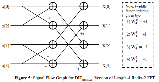
The DIT version of the radix-R FFT, where the input data set is ordered according to the DR mapping and the output data set according to the NAT mapping, is denoted hereafter by DIT_[DR,NAT] – see the example of Figure 5 where, from the SFG, it is evident that the powers of W4 must be ordered according to that of the output data set, namely via the NAT mapping. The stride for the first stage of butterflies has a value of one, whilst the stride for the second stage of butterflies has a value of two. Generalizing, for the case of a length-N radix-R FFT, the stride will increase from one stage to the next by means of a multiplicative scale factor of R, with the first stage having a value of one and the last stage having a value of N/R and the twiddle factors ordered according to that of the output data set, namely via the NAT mapping. Also, as with the case of the DIT_[NAT,DR] algorithm, the first stage involves just one set of N/R independent CU_R’s, all using the same set of R twiddle factors, whilst the second stage involves R sets, each of N/R2 independent CU ’s, with those CU ’s in each set R R using the same set of R twiddle factors. Continuing in this fashion, with the number of CU_R sets increasing from one stage to the next by a multiplicative scale factor of R, it is evident that the last stage involves N/R sets, each of just one CU_R, with that CU_R using its own distinct set of R twiddle factors (so that the last stage exploits all N twiddle factors).

The DIF Algorithm with Scrambled Output Data

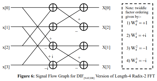
The DIF version of the radix-R FFT, where the input data set is ordered according to the NAT mapping and the output data set according to the DR mapping, is denoted hereafter by DIF_[NAT,DR] – see the example of Figure 6 where, from the SFG, it is evident that the powers of W4 must be ordered according to that of the input data set, namely via the NAT mapping. The stride for the first stage of butterflies has a value of two, whilst the stride for the second stage of butterflies has a value of one. Generalizing, for the case of a length-N radix-R FFT, the stride will decrease from one stage to the next by means of a multiplicative scale factor of 1/R, with the first stage having a value of N/R and the last stage having a value of one and the twiddle factors ordered according to that of the input data set, namely via the NAT mapping. Also, the first stage involves N/R sets, each of just one CU_R, with that CU_R using its own distinct set of R twiddle factors (so that the first stage exploits all N twiddle factors), whilst the second stage involves N/R2 sets, each of R independent CU ’s, with those CU_R’s in each set using the same set of R twiddle factors. Continuing in this fashion, with the number of CU_R sets decreasing from one stage to the next by a multiplicative scale factor of 1/R, it is evident that the last stage involves just one set of N/R independent CU_R’s, all using the same set of R twiddle factors.

The DIF Algorithm with Scrambled Input Data

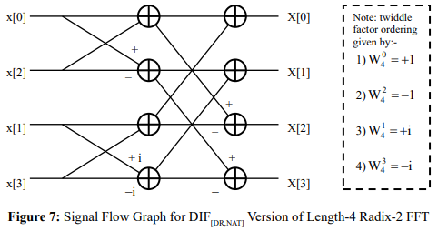
The DIF version of the radix-R FFT, where the input data set is ordered according to the DR mapping and the output data set according to the NAT mapping, is denoted hereafter by DIF_[DR,NAT] – see the example of Figure 7 where, from the SFG, it is evident that the powers of W4 must be ordered according to that of the input data set, namely via the BR mapping. The stride for the first stage of butterflies has a value of one, whilst the stride for the second stage of butterflies has a value of two. Generalizing, for the case of a length-N radix-R FFT, the stride will increase from one stage to the next by means of a multiplicative scale factor of R, with the first stage having a value of one and the last stage having a value of N/R and the twiddle factors ordered according to that of the input data set, namely via the DR mapping. Also, as with the case of the DIF_[NAT,DR] algorithm, the first stage involves N/R sets, each of just one CU_R, with that CU_R using its own distinct set of R twiddle factors (so that the first stage exploits all N twiddle factors), whilst the second stage involves N/R2 sets, each of R independent CU_R’s, with those CUR’s in each set using the same set of R twiddle factors. Continuing in this fashion, with the number of CU_R sets decreasing from one stage to the next by a multiplicative scale factor of 1/R, it is evident that the last stage involves just one set of N/R independent CU_R’s, all using the same set of R twiddle factors.

Discussion

Note that the term WN referred to in this section is that of the primitive Nth complex root of unity, as given by Equation 2, so that for the length-4 FFT examples provided

from which the required ordering of the twiddle factors for Figures 4 to 7 may be easily deduced. For ease of illustration, for the length-N transform, all N twiddle factors (including the trivial case,W_N⁰ ) derived from W_N are assumed here to have been pre-computed, stored N N and accessed using a suitably defined look-up table (LUT) – assumed here to be of length N, although it will be seen in the following section how far more efficient means of generating them might be obtained by exploiting those trigonometric symmetries present in the DFT definition. The stride parameter and the ordering of the twiddle factors for the radix-R FFT are as summarized in Table 1, where a scale factor of R implies that the stride value increases from stage to stage with an initial value of one and final value of N/R, whilst a scale factor of 1/R implies that the stride value decreases from stage to stage with an initial value of N/R and a final value of one. The associated number and size of distinct sets of independent CUR’s, per stage, are as summarized in Table 2, where a scale factor of R implies that the number of sets increases from stage to stage with an initial value of one and final value of N/R, whilst a scale factor of 1/R implies that the number of sets decreases from stage to stage with an initial value of N/R and a final value of one.

Algorithm Type	Stride Parameters First Stage       Last Stage		Scale Factor	Twiddle Factor Ordering
DIT[NAT,DR]	N/R	1	1/R	DR
DIT[DR,NAT]	1	N/R	R	NAT
DIF[NAT,DR]	N/R	1	1/R	NAT
DIF[DR,NAT]	1	N/R	R	DR

Table 1: Stride and Twiddle Factor Ordering Parameters for different Combinations of Decimation Scheme and Input/Output Data Ordering for Length-N Radix-R FFT

Algorithm Type	No of CUR Sets × No of CUR''s per Set First Stage                  Last Stage                 Scale Factor
DIT[NAT,DR]	1  × N/R	N/R × 1	R
DIT[DR,NAT]	1  × N/R	N/R × 1	R
DIF[NAT,DR]	N/R × 1	1  × N/R	1/R
DIF[DR,NAT]	N/R × 1	1  × N/R	1/R

Table 2: No of CUR sets and CUR’s per set for Different Combinations of Decimation Scheme and Input/Output Data Ordering for Length-N Radix-R FFT

With regard to the question of data reordering, it is evident that the computational complexity (which includes both arithmetic complexity and memory requirement) is the same for each of the four algorithmic variations discussed so that it is really a question of implementational convenience as to where the DR and NAT mappings should best be applied. If, for example, a forward transform was to be followed (after subsequent frequency-domain processing) by that of the corresponding inverse transform, then it would make sense to apply the DR in the frequency domain for the forward transform and in the time domain for the inverse mapping, as the combined effect of the two mappings (given that the DR mapping, as stated earlier, is its own inverse) would be that as produced by the identity mapping (or, effectively, to cancel each other out), thereby making their application in each domain unnecessary. Care would have to be taken, however, as any frequency-domain processing would be carried out on the scrambled version of the frequency-domain data, as produced by the forward transform.

Schemes for Efficient Generation of Twiddle Factors

The twiddle factors, as derived from the primitive Nth complex root of unity of Equation 2, are the data independent trigonometric coefficients that are input to the computational unit, CUR, where they are multiplicatively combined, in an appropriate fashion, with the corresponding components of the input data set. As stated in the introduction of Section 1, they comprise both sinusoidal and cosinusoidal terms which may be obtained from the use of one or more suitably sized LUTs. The amount of memory required by each LUT can be minimized by exploiting the relationship between the sine and cosine functions, as given by

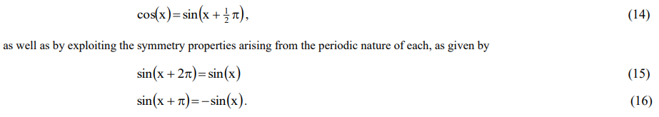
These relationships and properties are now exploited in Sections 4.1 and 4.2 so as to facilitate the development of LUT based storage schemes which may be optimized in order to minimize either: 1) the arithmetic complexity (of the addressing), at the expense of an increased memory requirement, or 2) the memory requirement, at the expense of an increased arithmetic complexity (of the addressing).

Also, given that for the radix-R FFT the CU_R requires, as input, the terms cos(n θ) and sin(n θ), for values of ‘n’ from 1 up to R-1, the terms may be obtained in an efficient manner via the use of standard multi-angle recursive formulae which may be combined with the use of one or more suitably sized LUTs to yield an additional approach to solving the problem of twiddle factor generation, as will be discussed in Section 4.3.

Minimizing Arithmetic Complexity

To minimize the arithmetic complexity for the generation of the twiddle factor addresses, a single LUT is best used with size according to a single quadrant addressing scheme [9], whereby the twiddle factors are read from a sampled version of the sine (or, equivalently, cosine) function with argument defined from 0 up to / 2 radians. As a result, the LUT may be accessed by means of a single, easy to compute, input parameter which may be updated from one access to another via simple addition using a fixed increment – that is, the addresses form an arithmetic sequence. Thus, for the case of a length-N FFT, it is required that the LUT be of length N/4, yielding a total memory requirement, denoted C_MEM , of

words. The corresponding arithmetic complexity, as expressed in terms of the required numbers of multiplications, denoted CMLT, and additions, denoted CADD, per twiddle factor, is given by

C_MLT = 0    & C_ADD = 2                                           (18)

respectively – that is, two additions for the generation of each twiddle factor, one for updating the LUT address of the sinusoidal component and one for that of the cosinusoidal component.

This single-level scheme described here would seem to offer, therefore, a reasonable compromise between the memory requirement and the addressing complexity, using more than the minimum achievable amount of memory required for the storage of the twiddle factors (albeit considerably less than would be required if the full 0 to 2π angular range was to be tabulated) so as to keep the arithmetic requirement of the addressing as simple as possible.

Minimizing Memory Requirement

When the transform to be computed is sufficiently long and the memory requirement thereby sufficiently large a multi-level LUT-based scheme [10], based upon the exploitation of multiple small single-level LUTs, might prove appropriate. The aim of such schemes is to reduce the memory requirement at the expense of increased arithmetic complexity with the twiddle factors being obtained from the contents of the multiple LUTs through the repeated application of the standard trigonometric identities

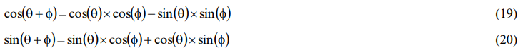
where θ corresponds to the angle defined over a ‘coarse-resolution’ angular region and to the angle defined over a ‘fine resolution’ angular region – see the simplified illustration of Figure 8 for the decomposition of the cosine function into coarse-resolution and fine-resolution angular regions, each of length 4.

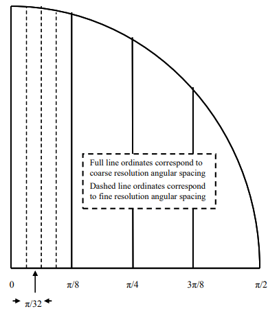
Figure 8: Decomposition of Single-Quadrant of Cosine Function into Coarse-Resolution & Fine-Resolution Angular Regions Using Single-Level Luts each of Length 4

Scheme Based Upon Multi-Level LUTs

Scheme Based Upon Second-Order Recursion

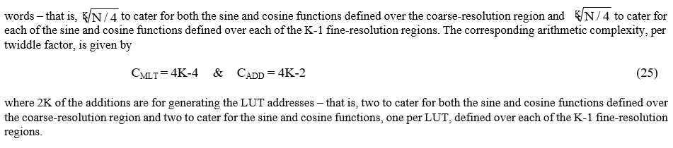
Note that after deriving the single-angle twiddle factor from one or more suitably sized LUTs, the remaining R-2 non-trivial multi-angle twiddle factors (noting that the first or zero-angle twiddle factor is trivial, being always equal to one) required by the radix-R FFT may be obtained directly from the single-angle angle twiddle factor through the application of the multi-angle recursive formulae, as given by

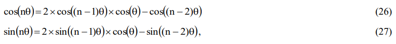
where ‘n’ is an arbitrary positive integer > 1. Such an approach to the computation of the non-trivial twiddle factors involves just two multiplications, two subtractions and two left-shift operations (each such operation being of length one, as used to implement multiplication by two) per twiddle factor. These two generic equations, which are both recursive equations of order two – each being commonly referred to as a second-order recursion or recurrence relation – enable each twiddle factor to be obtained directly from previously computed twiddle factors, in a simple recursive manner, rather than from one or more suitably sized LUTs.

Discussion

The memory requirement for the twiddle factor generation has been minimized through the exploitation of the periodic and symmetrical nature of the fundamental trigonometric functions from which the associated transform kernels are derived, namely the sine and cosine functions. The basic properties of these two complementary functions are as described by Equations 14 to 16 above, with the sinusoid being an even symmetric function relative to any odd-integer multiple of the argument / 2 and an odd symmetric function relative to any even integer multiple of / 2 , whilst the cosinusoid is an even-symmetric function relative to any even-integer multiple of the argument / 2 and an odd symmetric function relative to any odd integer multiple of / 2 . That is, they are each either even symmetric or odd symmetric according to whether the axis of symmetry is an appropriately chosen multiple of / 2 .

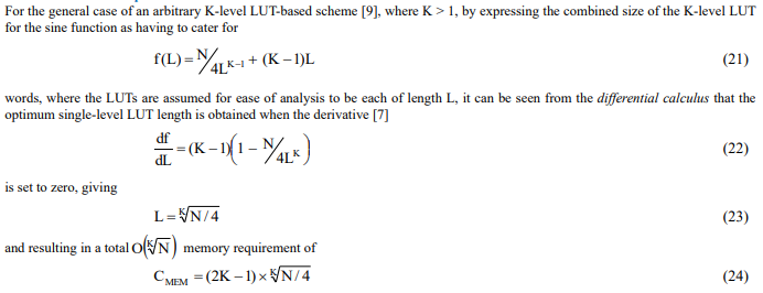
Note that the ideas discussed in this section have been dealt with in far more depth by the current author in [9], where parallel implementations are discussed for two particular twiddle factor generation schemes based upon the use of: 1) multi-level LUTs, and 2) the combined use of multi-level LUTs and second-order recursion. Although the multi-level LUT-based scheme has been illustrated in this section by means of the generic K-level scheme, for K > 1, in reality a two-level scheme would probably prove more than adequate for most signal processing applications of interest, involving the use of large to ultra-large orthogonal transforms such as the FFT [10], given that the memory requirement would reduce from O(N), as required for the single-level scheme, to just O(√N) for the two-level scheme, whilst the associated increase in arithmetic complexity would be minimal [9,10].

Parallel Computation of Fixed-Radix FFT Algorithm

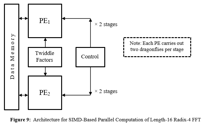
An attraction of the fixed-radix formulations of the FFT is that they lend themselves quite naturally to a parallel implementation. As has already been stated, the computation of the length-N radix-R FFT can be broken down into logRN stages, each of N/R independent CU_R’s, whereby the stages may be said to be defined over the temporal domain whilst the CU_R’s within any given stage may be said to be defined over the spatial domain. Note that whilst the CU_R relates to the set of repetitive arithmetic operations required to be computed by the FFT algorithm, with a hardware implementation in mind the processing element (PE) referred to hereafter relates to the associated hardware operators (such as logic-based adders and fast embedded multipliers, as provided by the computing device manufacturer) required for carrying out those operations. The remainder of this section looks briefly into how high-throughput parallel solutions to the fixed-radix FFT might be obtained by exploiting the inherent parallelism within each of these two domains. The techniques discussed are illustrated by means of a 16-point radix-4 FFT which comprises two stages with each stage involving the computation of four CU₄’s or dragonflies.

Coarse-Grain Parallelism for Spatial-Domain

A common way of achieving parallelization in the spatial domain is through the assigning of multiple identical PE’s for the coarse-grain parallel computation of the CU_R’s to be performed for each of the logRN stages of the length-N radix-R FFT. As the CU_R’s to be computed within each stage are independent of each other, requiring distinct R-fold input data sets, they may be carried out simultaneously via the single instruction multiple-data (SIMD) technique [4], which involves the assigning of a single instruction or set of instructions to each of the PE’s handling the processing of the multiple R-fold input data sets – see Figure 9. Given that each stage has to cater for the execution of N/R independent CU_R’s, such a scheme offers the possibility of achieving a maximum of N/R-fold parallelism, although when N is sufficiently large compared to R it might be more appropriate for each PE to handle multiple CU_R’s rather than a single CU_R. Thus, with such an approach, the number of tasks (and thus the amount of computation) to be performed by each PE, for any given stage, may potentially be quite large, ranging from one (whereby a single PE handles all the CU_R’s) up to N/R (whereby each CU_R is assigned its own PE) [11].

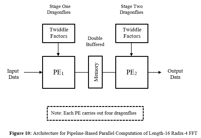
Coarse-Grain Parallelism for Temporal-Domain

By assigning an identical PE to each stage of processing, parallelization might be achieved in the temporal domain by having the multiple PE’s operating in a pipelined fashion [4], via a suitably defined computational pipeline of length logRN for the case of the length-N radix-R transform, with all the PE’s operating simultaneously, in a synchronous fashion, on their respective sets of independent CU_R’s. Note, however, that double-buffered memory (whereby the content of one memory is being processed whilst the content of the other is being created) must be provided between successive stages in order to prevent the occurrence of processing delays and thus to facilitate the continuous real-time operation of the pipeline – see Figure 10. Such an approach offers the possibility of achieving logRN-fold parallelism.

Fine-Grain Parallelism for Processing Element

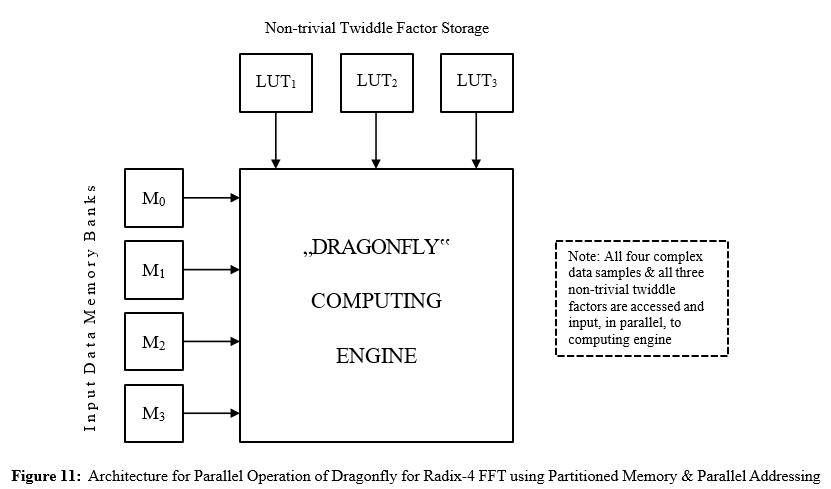
An additional level of parallelism to that described above in Sections 5.1 and 5.2 may be achieved through the exploitation of partitioned memory and parallel addressing for the parallel or simultaneous access of the R-fold input data set, thereby facilitating the fine-grain parallel computation, at the arithmetic level, of each individual CU_R . This involves the mapping of the input data set onto multiple equal-sized blocks of memory, or memory banks, as obtained from the partitioning of the available data memory – typically available in the form of fast random access memory (RAM) [12]. For the case of the multiple R-fold input data sets to the length-N radix-R FFT, for example, this might involve the construction of R banks of dual-port memory (whereby one complex sample of data might be simultaneously obtained from each memory bank), each capable of storing N/R complex words. For the R complex samples of data (as required for input to each instance of the CU_R) to be accessed simultaneously and unambiguously from the R memory banks, however, it will be necessary that potential addressing conflicts be avoided. In order to achieve this, a circular addressing scheme [14] could be adopted which simply rotates the memory bank addresses, so that the data samples for each R-fold input data set will be located in different memory banks. Such a scheme offers the possibility of achieving R-fold parallelism, so that the larger the transform radix the larger the potential achievable parallelism.

The much simpler problem relating to the storage and access of the twiddle factors could be solved very simply by assigning a separate single-level or multi-level LUT for each of the R-1 non-trivial twiddle factors, thereby enabling all the twiddle factors to be simultaneously available for input to the CU_R. Clearly, when the R-fold input data set, as well as the set of twiddle factors, are simultaneously available for input to the CU_R, as is illustrated in Figure 11, then the PE may be operated in parallel, thereby facilitating the introduction of fine-grain parallelism into the computation of the CU_R, whereby the individual tasks to be carried out are relatively small involving simple adders and multipliers.

Discussion

The partitioned memory and the associated parallel addressing may clearly be beneficially used in the design of a highly-parallel PE which could then be exploited by either SIMD (using one or multiple PE’s) or pipelined approaches to the parallelization of the fixed-radix FFT (and, in addition, for those parallel pipelined solutions involving the combined use of both SIMD and pipelined processing techniques). With regard to the spatial-domain and temporal-domain processing, the coarse-grain parallelism of the SIMD and pipelined approaches may each achieve highly-parallel solutions but only at the expense of requiring increased resources in terms of increased arithmetic and memory. It should be noted, however, that if the transform radix is sufficiently large, then adequate performance might also be achieved, at greatly reduced cost, via the adoption of a single highly-parallel PE, using double-buffered partitioned memory and parallel addressing to achieve fine-grained parallelism. For each of these techniques, there will be constraints placed upon the achievable performance arising from the choice of computing device. With the adoption of field programmable gate array (FPGA) technology [12], for example, a performance metric based loosely upon the maximizing of the computational density (that is, maximizing the throughput per unit area of silicon) or the related problem of minimizing the power requirement (that is, minimizing the required silicon area and/ or clock frequency), might yield an appropriate choice of computing architecture, such as the simplified design of the scalable memory-based architecture for minimizing the resource requirement or the pipelined architecture for maximizing the computational throughput, with each solution being subject to certain constraints upon the available resources (such as those of update time, memory requirement or arithmetic complexity, for example). A comparison of solutions, based upon the adoption of these two architectures, for the parallel computation of the real-data version of the fixed-radix FFT is given in [8], whilst a comparison of parallel solutions to the problem of twiddle factor generation for the fixed-radix FFT is given in [11].

Summary and Conclusion

This paper, which is of a tutorial nature, has been concerned with the computation of the generic radix-R version of the fixed-radix FFT algorithm, where R is taken to be an arbitrary positive integer. Much of the existing technical literature on the fixed-radix FFT deals with those simple cases where the radix takes on a value of either two or four and where certain restrictions are assumed on the placement of the index mappings. To address this situation, four algorithmic variations have been discussed here for dealing with the radix-R FFT, these arising from the adoption of different combinations of decimation scheme, as provided by the DIT and DIF techniques, and data reordering scheme, as provided by the NAT and DR index mappings. The computational unit, CU_R, as required for the efficient computation of the repetitive arithmetic operations required by the radix-R transform, has been described here in some detail for all four variations. To provide a good understanding of the operation of the CU_R, the detailed descriptions of three key concepts have been provided, namely: 1) the R-fold input/output data set, relating to the independent output data sets produced from distinct input data sets by the CU_R; 2) the stride, relating to the stage-dependent address spacing of the R-fold interleaved (and thus independent) input data sets to the CU_R; and 3) the number and size of distinct sets of independent CU_R’s, per stage, each set requiring its own distinct set of R twiddle factors. These concepts have been illustrated through the provision of detailed examples for each of the four algorithmic variations where a transform length of four has been assumed for ease of illustration. Finally, a brief account has been given of those techniques – as defined over both spatial and temporal domains – that could be exploited in order to facilitate the efficient parallel computation of the radix-R FFT when suitably defined parallel equipment is available for its implementation. This has involved SIMD and pipelined processing techniques together with the parallel addressing of data stored in partitioned memory in order that both data and twiddle factors might be simultaneously accessed for the parallel input to the CU_R .

Conflicts of Interest: The author, having been retired for some years, has no access to funding of any kind and states that there are no conflicts of interest associated with the production of this paper.

References

1. Ahmed, N., & Rao, K. R. (2012). ‘‘Orthogonal transforms for digital signal processing’’. Springer Science & Business Media.
2. G. Birkhoff & S. MacLane, “A Survey of Modern Algebra”, Macmillan, 1977.
3. McClellen, J. H., & Rader, C. M. (1979). Number theory in digital signal processing. Prentice Hall Professional Technical Reference.
4. S.G. Akl, “The Design and Analysis of Parallel Algorithms”, Prentice-Hall, 1989.
5. E. Chu & A. George, “Inside the FFT Black Box: Serial and Parallel Fast Fourier Transform Algorithms”, CRC Press, 2000.
6. D.F. Elliott & K.R. Rao, “Fast Transforms: Algorithms, Analyses, Applications”, Academic Press, 1982.
7. G.H. Hardy, “A Course of Pure Mathematics”, Cambridge University Press, 1928.
8. K.J. Jones, “A Comparison of Two Recent Approaches, Exploiting Pipelined FFT and Memory Based FHT Architectures, for Resource-Eficient Parallel Computation of Real-Data DFT”, Journal of Applied Science and Technology (OPAST Open Access), Vol. 1, No. 2, July 2023.
9. K.J. Jones, “Schemes for Resource-Eficient Generation of Twiddle Factors for Fixed-Radix FFT Algorithms”, Engineering (OPAST Open Access), Vol. 2, No. 3, July 2024.
10. K.J. Jones, “Design of Scalable Architecture for Real-Time Parallel Computation of Long to Ultra Long Real-Data DFTs”,Engineering (OPAST Open Access), Vol. 2, No. 4, November 2024.
11. K.J. Jones, “A Comparison of Two Schemes, Based upon Multi-Level LUTs and Second Order Recursion, for Parallel Computation of FFT Twiddle Factors”, Trans. on Applied Science, Engineering and Technology (Open Access), Vol. 1, No. 1, July 2025.
12. Maxfield, C. (2004). The design warrior’s guide to FPGAs: devices, tools and flows. Elsevier.
13. E.O. Brigham, “The Fast Fourier Transform”, Prentice-Hall, 1974.
14. Reisis, D., & Vlassopoulos, N. (2008). ‘‘Conflict-free parallel memory accessing techniques for FFT architectures’’. IEEE Transactions on Circuits and Systems I: Regular Papers, 55(11), 3438-3447.
15. Stockham Jr, T. G. (1966, April). ‘‘High-speed convolution and correlation’’. In Proceedings of the April 26-28, 1966, Spring joint computer conference (pp. 229-233).