A Simple Algorithm for Converting Random Number Generator Outputs to Universal Distributions to Aid Teaching and Research in Modern Physical Chemistry

Introduction

Modeling that utilizes probability and randomness employs the concept of random numbers to achieve statistical explanations of complex physical phenomena, such as the stochastic equation of motion and kinetic Monte Carlo models. Monte Carlo simulations represent a large class of computational algorithms and experiments that allow one to use repeated random sampling to probe complex processes and dynamics. Monte Carlo modeling has been extensively applied to complex chemical problems, such as electronic structures, molecular dynamics, statistical thermodynamics, and quantum optics, all of which are central to both classical and modern physical chemistry education. Techniques such as Monte Carlo widely utilize random numbers generated using standard “black box” algorithms. In this article, we describe a simple algorithm that relates random number generation to the real probability distribution of any single variable. Probability distributions are broadly covered in undergraduate chemistry classes, but the link to stochastic simulations is rarely made. Hence, our proposed tool, while broadly accessible to undergraduate students, links the content of physical chemistry courses to outcomes of stochastic simulations and helps overcome the student- experienced barrier to computer simulations for chemical problems. The method can be directly used in the classroom education of statistical thermodynamics and assist physical chemistry undergraduate and graduate students in related fields with modeling analysis [1-8].

We will briefly introduce the standard analytical approach to converting evenly distributed random numbers into any arbitrary distribution, which we call the Random Number Converter (RNC), though it is commonly named inverse transform sampling. We begin with the example of a single-exponential decay distribution, PDF (x) = ke^-kx, where PDF stands for probability density function, and ÃÂ? is a real number. This exponential distribution represents varied behavior, such as the time difference between random events that occur with a given frequency. It is also known as the zeroth-order Poisson distribution. To relate a random number valued between 0 and 1 to this PDF, we must evaluate the cumulative distribution function (CDF), which measures the area under the curve as a function of the position along the curve. Single-exponential decay distributions have an analytical cumulative distribution function, i.e., CDF(x) = ^x f(x′) dx′ is the closed-form function,

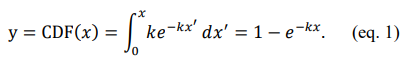
This function can then be inverted (i.e. x can be expressed as a closed-form function in terms of y), which allows us to derive the analytical inverse CDF,

Here, x can be the vector to store our desired random numbers that follow the single-exponential decay PDF, where is a uniform random vector ranging between 0 and 1 that can be called from a pseudorandom number generator in all conventional programming languages [2,8,9].

We see that in the foresaid example, the random numbers are straightforwardly drawn from a closed-form inverse CDF. However, generating random numbers for any PDF presents two main difficulties: (i) the corresponding CDF often lacks an analytical solution, and (ii) the inverse function of the CDF is often not analytic. These challenges are addressed computationally with a number of methods common in numerical simulation, such as kernel density estimation and Markov chain Monte Carlo. As a result, the implementation and interpretability of algorithms are hindered, creating a barrier to student learning and connecting simulations and chemistry. Here we present our RNC as a simple numerical algorithm based on inverse transform sampling to convert uniform random numbers. Implementation of this algorithm provides multiple steps and opportunities for pedagogical explanation of modern concepts in chemical simulation and allied fields, such as statistics, computer science, materials science, chemical engineering, biology, and more. In the following, we will explore the intended learning outcomes (ILOs) and how RNC serves as a versatile tool for demystifying complex probability distributions, providing students with a hands-on learning experience that transcends traditional classroom instruction [10-13].

Intended Learning Outcomes

• Grasp Probability Distributions and Stochastic Techniques

students will gain a solid understanding of probability distributions and learn how to apply stochastic sampling methods, such as Monte Carlo simulations.

• Master the RNC Algorithm

students will become proficient in using the RNC algorithm to transform uniformly

Figure 1: Graphic summary of the ILOs of RNC implementation in modern physical chemistry. Distributed random numbers into universal PDFs.

• Develop Skills in Analyzing and Simulating Chemical Data

students will learn to analyze and simulate spectroscopy and visualize reaction kinetics using computational techniques, including the RNC algorithm.

• Link Abstract Mathematics to Practical Simulations

students will develop a deeper understanding of abstract physical chemistry mathematics by interpreting results from stochastic simulations and linking them to practical applications.

• Integrate Multidisciplinary Knowledge

students will cultivate the ability to integrate concepts from statistics and computer science to understand physical chemical phenomena.

• Enhance Computational and Programming Skills

students will improve their computational and programming abilities, particularly in MATLAB and Python, enabling them to understand the limitations and assumptions inherent in various modeling approaches.

Results and Discussion

The Schematic Procedure of Our RNC

The method is detailed in Figure 2, and the MATLAB and Python scripts with comments are provided in Section 1 of the Supporting Information (SI). Firstly, for any given PDF, we numerically integrate it to obtain the CDF using the trapezoidal method, where 10⁴ to 10⁵ x-grid points for the PDF are enough (i.e. there are the same number of PDF and CDF y-grid points). This decision aims to help undergraduate students grasp the process and ease the transition to other programming languages, such as C or Fortran, for researchers incorporating this RNC module into their research. Educators could use this as a chance to describe other numerical integration methods, such as Riemann sums or Simpson’s rule, or more sophisticated methods, such as Gaussian quadrature or Monte Carlo integration algorithms [14-,15].

Figure 2: Scheme of the RNC method, where a given PDF is inputted, the CDF is computed numerically, both are normalized, the inverse CDF is obtained through binary search, and a set of random numbers that follow the desired PDF is obtained. A typical Maxwell-Boltzmann PDF example is shown on the right.

The grid density and number of bins could be tested by the students as an exercise, experimenting with the algorithm’s behavior and convergence Next, a constant-probability random number, _i, between 0 and 1 is obtained to describe a random probability. We note that this provides an additional opportunity to discuss methods for random number generation, such as the idea of pseudorandom numbers and the need for methods to generate truly random numbers, as recently highlighted in the active area of quantum research. A function value of the CDF (i.e. y = CDF (x) value) closest to this random probability is then picked using a binary search solution to numerically achieve the process of obtaining the inverse of the CDF. Once again, another opportunity is presented here to discuss search algorithms and their relative efficiencies. Finally, the x_i value corresponding to the selected CDF value is determined, representing one of the desired random numbers. With multiple _i inputs, a set of x_i (i.e. {x_i}) is obtained and stored, where the histogram of {x_i} fully reproduces the desired PDF. In Figure 2, a typical Maxwell-Boltzmann distribution (i.e. PDF (x) = Ax²−e^-x, where A is the normalization factor) is shown as an illustration. To facilitate hands-on exploration, students can adjust parameters, such as the number of bins, grid spacing, and value of k, and experiment with additional factors, such as the method of interpolation or introduction of noise, offering a dynamic platform to understand the nuances of shaping random numbers into various PDFs. Hereinafter, we show the use of this RNC in different cases [16].

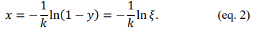
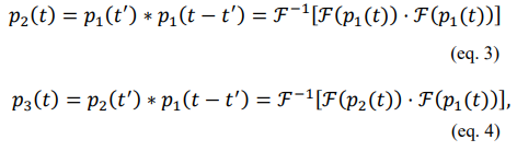
Common distribution shapes: In Figure 3(a), we demonstrate for the previously mentioned single-exponential decay distribution, PDF (x) = ke^-kx, that, without any of the algebraic work, our numerical method can obtain random numbers with the desired distribution shape. Here, we choose k = 1 for simplicity, and 107 random numbers and its corresponding histogram with 100 bins were created. The normalized PDF and CDF are plotted as well. We also show the analytical results in Section 2 of the SI as a direct comparison. The Gaussian PDF is another important distribution used in both statistical and quantum mechanics due to its relationship with the central limit theorem A Gaussian has a CDF that involves the error function, which is not a closed-form function (i. e. it cannot be expressed without using infinite summation). The typical algorithm of obtaining Gaussian-distributed random numbers is through the Marsaglia polar method, which utilizes the Box-Muller transform (example in Section 3 of the SI) In Figure 3(b), we illustrate that our method can also capture such a distribution with an example

More complicated distribution shapes: In the real world, distributions of physical quantities such as time, force, velocity, position, energy, etc. for a system are usually not ideal single-exponential or normal Gaussian shapes [5,8,22-26]. The presented method i designed to tackle such situations. In Figure 

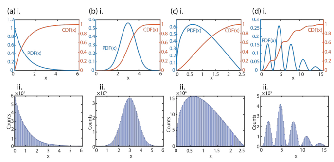
Figure 3 (a) i. Normalized PDF and the corresponding CDF (numerically obtained) of a single-exponential decay distribution.ii. 100-bin histogram of 107 random numbers obtained from the binary search method that follows the single-exponential decay distribution. (b) i. and ii. are the same as (a) i. and ii., but for a typical Gaussian distribution. (c) i. and ii. are the same as (a) i. and ii., but for a sine function-based distribution. (d) i. and ii. are the same as (a) i. and ii., but for a more complicated distribution shape that combines polynomial, exponential, and sine functions.

substitution, the CDF is still analytically achievable. However, the inverse CDF is a transcendental equation that permits multiple solutions. Nevertheless, with our binary search of the numerically obtained CDF, the shape can betreated as a common distribution and obtained in a straightforward manner. In Figure 3(d), a more extreme case is shown, where the PDF (x) = x²e^-x\2(sin x)² contains polynomial, exponential, and sine functions. Here, the CDF and its inverse both become challenging. However, with the presented method, the random numbers can be easily obtained.

Rate of a catalytic turnover cycle (F1-ATPase model): Through step-by-step demonstrations and interactive exercises, educators can illustrate how RNC empowers learners to tailor random number outputs to specific distributions, facilitating a deeper grasp of physical chemistry concepts. Utilizing our RNC, complicated chemical reaction kinetics can be analyzed easily without any additional algebra. This can help students numerically convince themselves of theoretically.

Figure 4 (a). The F1-ATPase “rotary motor” reaction scheme. (b). PDFs of the time, t, to go from state 1 back to state 1 (i.e. the full catalytic turnover cycle) with respect to different ATP concentrations, [ATP], ranging from 0. 1 to 0. 3 M. Here, the single-step (i.e. i to i + 1) rate, k, is assumed to be 5 M⁻¹s⁻¹. (c). Illustrations of histograms of 10⁶ random times created by the presented RNC for [ATP] = 0.1, 0.2, and 0.3 M with 100 bins each. (d). Calculated sample means, [t]cycle, from the random times with standard deviations at each T = (K[ATP]) point. These average times are linearly fitted to obtain a slope of 2. 995.

derived solutions. Here, we use F1-ATPase as a simple model. F1-ATPase is a “rotary motor” consisting of three dimeric subunits (i.e. states 1, 2, and 3) that act as a “stator”. The central unit does a complete turn upon sequential binding to one of the subunits of ATP, performs hydrolysis, and releases ADP. This catalytic turnover cycle is schematized in Figure 4(a). Here, we let k be the ATP binding rate constant. The time, t, to go from state i to i ? + 1 (i.e. a single-step) is distributed randomly with a mean time,  T = 1⁄ (k [ATP]), and a single-exponential decay distribution, _p1(t) = e^-t\T , where [ATP] is the molar concentration of ATP (k is in units of M−1s−1). The single-step reaction is second-order with respect to the reactant concentration. Since the reaction occurs sequentially over time, the total turnover time (i.e. going from state i back to state i) distribution is represented as successive convolutions of the single-step reaction [35-37].

To numerically obtain the distribution of turnover times and avoid analytically solving the convolutions, we evaluate it computationally using the convolution theorem based on Fourier transforms (Blackwell and Simpson, n.d.). Therefore, the two-and three-step distributions (i.e. p2 and p3, respectively) are

where “ ∗ ” indicates the convolution and F and F⁻¹ represent Fourier and inverse Fourier transforms, respectively. The PDFs with different [ATP] ranging from 0. 1 to 0. 3 M are illustrated in Figure 4(b) with k set to be 5 M−1s−1. The 100-bin histograms of 106 random times obtained from our RNC associated with [ATP] of 0.1, 0.2, and 0.3 M are shown in Figure 4(c). With several samples among different [ATP] values, the mean turnover times,[t]_cycle, and the sample standard deviations are calculated. In Figure 4(d), with a linear fitting, we obtain a slope of 2. 995 (i. e.[t]_cycle ~3_^T where the mean turnover time is simply three times that of a single-step and linearly related to 1/[ATP]). This result aligns precisely with the analytically derived solutions (Section 4 of the SI), thereby showing that this RNC can help students intuitively see the rules of chemical reaction kinetics. Together with the analytical derivation, students can better understand its physical and chemical principles. Furthermore, it illustrates how stochastic processes can lead to changes in distributions, but not changes in average properties.

Colored photon streams for interferometric analysis: Another example is numerical analysis in spectroscopy. When performing spectroscopic experiments of chemical compounds, multiple physical processes can occur simultaneously. The resulting emission spectrum may represent different emissive populations, energy transfer between states, and linewidth broadening resulting from excited state fluctuations. For such non- standard PDF shapes (i.e. emission spectra), our RNC allows one to “sample” photon energies and describe how they may propagate through an optical experiment, such as filters, dichroic mirrors, and interferometers. Here, we propose two mock emitters, a “red” one with a peak emission of ~1.25 eV and a “blue” one with a peak emission of ~1.35 eV. The photoluminescent (PL) spectrum is assumed to carry a skewed Gaussian with Lorentzian shape, where the skewness (i.e. asymmetry) is designed to account for the possible deviations of the relaxation pathways of each individual emitting molecule [27-32].

The simulated spectra are shown in Figure 5(a)i. One possible single-emitter PL function could be

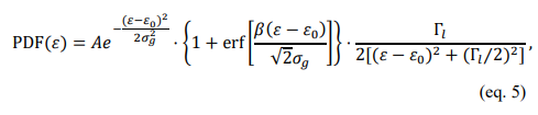
where A is the overall normalization constant, £0 is the peak emission energy, g is the standard deviation of the Gaussian distribution that is equal toto  Γ_g/(2√2 ln 2) , Γ_g is the Gaussian full-width at half maximum (FWHM), Γ_n is the Lorentzian FWHM, and ß is the skewness parameter, where a larger number results in a more skewed spectrum and a positive or negative ß indicates left or right skewness, respectively. Therefore, for each emitter type, we can supply a set of spectral parameters, {£₀, Γ_g, Γ_l, ß}. Here, we used {1. 25, 0. 40, 0. 16, −6} for the “red” emitter and {1. 35, 0. 18, 0. 08, −3} for the “blue” emitter.

The PL spectrum can be thought of as a photon counting statistics of colors, where we can acquire random colors for each simulated photon that satisfies the PL line shape in eq. 5. Obviously, obtaining an analytical CDF or inverse CDF is impossible. Here, we illustrate the results (i.e. CDF and the created histograms) using our numerical method in Figure 5(a) ii. and iii. With these colors.

Figure 5 (a) i. Simulated dual-emitter PL spectra where both “red” and “blue” emitters are assumed to have the product of a skewed Gaussian and Lorentzian line shape. ii. Corresponding CDFs. iii. Histogram of obtained random numbers (i.e. colors of photons) that follow the given PL spectra. (b) i. and ii. Simulated MZI against the stage positions (scan ± 50 mm) for the isolated “red” and “blue” emitters and their Fourier transformed spectra. (c). Simulated MZI for the combined “red” and “blue” emitters as a total interferogram. Fourier transformed spectra for the total interferogram (black) with the isolated ones (red and blue).

statistics, we can further use these random numbers for spectral analysis. Atallah et al. presented in their work the single-photon counting interferometry using the Mach-Zehnder interferometer (MZI), which can be considered as a cosine filter in the frequency domain. Therefore, our random colors can be used to retrospectively generate MZI interferograms (Section 5 of the SI). Photon streams, assuming perfectly Poisson emission (i.e. single-exponential decay distribution in time), with colored photons are sent to the cosine filter. Photons are then directed (i. e. self-interfere) to end up probabilistically favoring a detector (i.e. D1 or D2). Interference effects then result in a given perfectly anticorrelated probability, (p). Here,

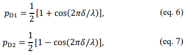
where null  is the movable delay stage position in the interferometer (i.e. the relative photon arrival path length) and = hc/£ is the photon wavelength (i.e. color). The photon counting outcomes at each detector with respect to a specific stage position, , represents the signal intensities, S_D1() and S_D2(). Therefore, the total anticorrelated signal intensity, S() , is In single-emitter cases (i.e. only “red” or only “blue” emitters are present), the interferograms against the stage positions are shown in Figure 5(b) and overlaid with the single-sided Fourier transforms of the interferograms, which excellently reproduce the given initial PDFs. In Figure 5(c)i. and ii., the mixed-emitter case is illustrated, where a stream of mixed-color photos from “red” and “blue” emitters are constructed. The total interferogram and its Fourier transform are shown. The Fourier transformed line shape shows perfect agreement with the given PL spectrum, demonstrating that our simple RNC can be used by students or researchers to conduct retrospective analysis and simulation of Fourier spectroscopy [19,34].

In the classroom setting, hands-on activities utilizing RNC can provide students with valuable insights into the significance of probability distributions in simulating real-world chemical phenomena. Through intuitional simulation with RNC, complex processes become visually accessible without the need for heavy algebraic computations. By incorporating RNC into laboratory experiments, students can actively engage in the process of generating data that adheres to predetermined distribution functions, enhancing their experimental skills and analytical prowess [38].

Conclusion

In this work, we introduce a very simple RNC capable of converting uniform random numbers to any given real distribution shape (i.e. PDF). It utilizes a numerical scheme to obtain the CDF, avoiding the possibly algebraically difficult analytical integration. After obtaining the CDF, we employ the binary search method to obtain the corresponding random numbers, bypassing the need of computing the inverse CDF as most functions lack an analytical inverse (i.e. inverse transform sampling). We demonstrate its application for simple distributions, such as exponential and Gaussian distributions, and its handling of more complicated PDFs, such as combined trigonometrical and polynomial functions. Finally, we illustrate its application in the analysis of chemical reaction kinetics and Fourier spectroscopy. In the catalytic turnover F1-ATPase reaction model, we demonstrate the capability of our RNC in obtaining the relation between the mean turnover time, single-step rate, and concentration of ATP without heavy algebraic work. This provides an easy and intuitive way for students to visualize the analytically derived reaction kinetics results. In the example of Fourier spectroscopy, we illustrate the analysis by assigning a random color to simulated photons with the distribution pattern determined using hypothesized spectra. This allows for retrospective interferometry analysis, which is useful for teaching spectroscopy courses and conducting Fourier spectroscopy modeling and analyses. Numerous derivatives and developments can emerge from this simple method. For instance, the current RNC code is limited by hardware memory. More implementation can be done to not only augment computing speed but to also mitigate memory costs, thereby optimizing computational efficiency. However, we believe that the integration of these algorithms provides a platform to teach basic concepts in computer science, such as memory management, hardware constraints, and numerical integration methods as they have become more crucial in modern physical chemistry. Additionally, discussions on more sophisticated search algorithms can be incorporated, enriching students' understanding of algorithmic design principles and their applications. Moreover, extending the RNC module to other programming languages such as Maple and Mathematica is imperative. These languages, renowned for their pedagogical value, offer hands-on opportunities to explore statistical concepts, such as distributions, histograms, and sampling. By leveraging these tools, educators can provide comprehensive instruction on random number conversion techniques while fostering a deeper understanding of computational efficiency and statistical methodologies among physical chemistry students.

Overall, we believe that our simple method for converting random number generator outputs to universal distribution shapes offers versatile applications in teaching and research in physical chemistry. Utilizing this RNC not only simplifies the conversion process but also instills a sense of confidence and proficiency among students as they navigate the intricacies of probability theory and statistical analysis. The intuitive nature of the RNC algorithm makes it a valuable tool for educators seeking to elucidate complex concepts surrounding probability distribution functions, offering students a tangible means of conceptualizing abstract mathematical principles. This interdisciplinary implementation results in hands-on learning outcomes, helping students adapt to advanced physical chemistry courses, industrial applications, and academic research. Through continuous refinement and integration into pedagogical frameworks, RNC, alongside its integration with Monte Carlo simulations, holds the potential to revolutionize the way students and researchers approach the synthesis and analysis of data in the field of physical chemistry.

References

1. Khirich, G. (2021). A Monte Carlo method for analyzing systematic and random uncertainty in quantitative nuclear magnetic resonance measurements. Analytical Chemistry, 93(29), 10039-10047.
2. Lecca, P. (2013). Stochastic chemical kinetics: A review of the modelling and simulation approaches. Biophysical reviews, 5, 323-345.
3. Lin, S. H., & Eyring, H. (1974). Stochastic processes in physical chemistry. Annual Review of Physical Chemistry, 25(1), 39-77.
4. Okada, K., Brumby, P. E., & Yasuoka, K. (2021). An efficient random number generation method for molecular simulation. Journal of Chemical Information and Modeling, 62(1), 71-78.
5. Stacklies, W., Seifert, C., & Graeter, F. (2011). Implementation of force distribution analysis for molecular dynamics simulations. Bmc Bioinformatics, 12, 1-5.
6. Oliveira, C. J., dos Santos, M. T., & Vianna Jr, A. S. (2022). A proposal to cover stochastic models in chemical engineering education. Education for Chemical Engineers, 38, 86-96.
7. Ringer McDonald, A. (2021). Teaching Programming across the Chemistry Curriculum: A Revolution or a Revival? In Teaching Programming across the Chemistry Curriculum (pp. 1-11). American Chemical Society.
8. Fisher, B. R., Eisler, H. J., Stott, N. E., & Bawendi, M.G. (2004). Emission intensity dependence and single-exponential behavior in single colloidal quantum dot fluorescence lifetimes. The Journal of Physical Chemistry B, 108(1), 143-148.
9. Tanabe, T. (1998). Photon statistics of various radiation sources. Nuclear Instruments and Methods in Physics Research Section A: Accelerators, Spectrometers, Detectors and Associated Equipment, 407(1-3), 251-256.
10. WÃÃÂ???glarczyk, S. (2018). Kernel density estimation and its application. In ITM web of conferences (Vol. 23, p. 00037). EDP Sciences.
11. Wu, L., Ji, W., & AbouRizk, S. M. (2020). Bayesian inference with Markov chain Monte Carlo–based numerical approach for input model updating. Journal of Computing in Civil Engineering, 34(1), 04019043.
12. Devroye, L. (2006). Nonuniform random variate generation. Handbooks in operations research and management science, 13, 83-121.
13. Batstone, D. J. (2013). Teaching uncertainty propagation as a core component in process engineering statistics. Education for Chemical Engineers, 8(4), e132-e139.
14. Ma, J., Rokhlin, V., & Wandzura, S. (1996). Generalized Gaussian quadrature rules for systems of arbitrary functions. SIAM Journal on Numerical Analysis, 33(3), 971-996.
15. Song, C., & Kawai, R. (2024). Sampling and change of measure for Monte Carlo integration on simplices. Journal of Scientific Computing, 98(3), 64.
16. Liu, W. B., Lu, Y. S., Fu, Y., Huang, S. C., Yin, Z. J., Jiang,K., ... & Chen, Z. B. (2023). Source-independent quantum random number generator against tailored detector blinding attacks. Optics Express, 31(7), 11292-11307.
17. Maragó, O. M., Bonaccorso, F., Saija, R., Privitera, G., Gucciardi, P. G., Iatì, M. A., ... & Ferrari, A. C. (2010). Brownian motion of graphene. ACS nano, 4(12), 7515-7523.
18. Shy, L. Y., & Eichinger, B. E. (1986). Shape distributions for Gaussian molecules: circular and linear chains in two dimensions. Macromolecules, 19(3), 838-843.
19. Mandal, K. (2022, August). Cryptographic Pseudorandom Noise Generators for Lattice-based Cryptography and Differential Privacy. In 2022 10th International Workshop on Signal Design and Its Applications in Communications (IWSDA) (pp. 1-4). IEEE.
20. Marsaglia, G. (1991). Normal (Gaussian) random variables for supercomputers. The Journal of Supercomputing, 5(1), 49-55.
21. Marsaglia, G., & Bray, T. A. (1964). A convenient method for generating normal variables. SIAM review, 6(3), 260-264.
22. Gentekos, D. T., & Fors, B. P. (2018). Molecular weight distribution shape as a versatile approach to tailoring block copolymer phase behavior. ACS Macro Letters, 7(6), 677-682.
23. Laimer, F., Zappa, F., & Scheier, P. (2021). Size and velocity distribution of negatively charged helium nanodroplets. The Journal of Physical Chemistry A, 125(35), 7662-7669.
24. Long, C., Dong, Z., Yu, F., Wang, K., He, C., & Chen, Z.R. (2023). Molecular weight distribution shape dependence of the crystallization kinetics of semi crystalline polymers based on linear unimodal and bimodal polyethylenes. ACS Applied Polymer Materials, 5(4), 2654-2663.
25. Nguyen, V. T., & Papavassiliou, D. V. (2021). Velocity magnitude distribution for flow in porous media. Industrial & Engineering Chemistry Research, 60(38), 13979-13990. 
26. Woo, S. J., & Kim, J. J. (2021). TD-DFT and experimental methods for unraveling the energy distribution of charge-transfer triplet/singlet states of a tadf molecule in a frozen matrix. The Journal of Physical Chemistry A, 125(5), 1234-1242.
27. Alivisatos, A. P., Harris, A. L., Levinos, N. J., Steuerwald, M. L., & Brus, L. E. (1988). Electronic states of semiconductor clusters: Homogeneous and inhomogeneous broadening of the optical spectrum. The Journal of chemical physics, 89(7), 4001-4011.
28. Riesen, H. (2006). Hole-burning spectroscopy of coordination compounds. Coordination chemistry reviews, 250(13-14), 1737-1754.
29. Cury, L. A., Guimaraes, P. S. S., Moreira, R. L., & Chacham,H. (2004). Asymmetric line shape in the emission spectra of conjugated polymer thin films: An experimental signature of one-dimensional electronic states. The Journal of chemical physics, 121(8), 3836-3839.
30. Gao, Y., & Yin, P. (2017). Origin of asymmetric broadening of Raman peak profiles in Si nanocrystals. Scientific Reports, 7(1), 43602.
31. Toutounji, M. (2019). Linear and nonlinear Herzberg-Teller vibronic coupling effects. I: Electronic photon echo spectroscopy. Chemical Physics, 521, 25-34.
32. Wang, Z., Wang, Z., Ling, F. C., & Su, Z. (2022). Asymmetric Broadening and Enhanced Photoluminescence Emission in ZnO Due to Electron–Phonon Coupling. The Journal of Physical Chemistry C, 126(32), 13814-13820.
33. Atallah, T. L., Sica, A. V., Shin, A. J., Friedman, H. C., Kahrobai, Y. K., & Caram, J. R. (2019). Decay-associated fourier spectroscopy: visible to shortwave infrared time-resolved photoluminescence spectra. The Journal of Physical Chemistry A, 123(31), 6792-6798.
34. Sica, A. V., Hua, A. S., Lin, H. H., Sletten, E. M., Atallah,T. L., & Caram, J. R. (2023). Spectrally Selective Time-Resolved Emission through Fourier-Filtering (STEF). The Journal of Physical Chemistry Letters, 14(2), 552-558.
35. Okazaki, K. I., & Hummer, G. (2013). Phosphate release coupled to rotary motion of F1-ATPase. Proceedings of the National Academy of Sciences, 110(41), 16468-16473.
36. Steel, B. C., Nord, A. L., Wang, Y., Pagadala, V., Mueller,D. M., & Berry, R. M. (2015). Comparison between single-molecule and X-ray crystallography data on yeast F1-ATPase. Scientific Reports, 5(1), 8773.
37. Stewart, A. G., Sobti, M., Harvey, R. P., & Stock, D. (2013). Rotary ATPases: models, machine elements and technical specifications. Bio architecture, 3(1), 2-12.
38. Blackwell, C. A., & Simpson, R. S. (1966). The convolution theorem in modern analysis. IEEE Transactions on Education, 9(1), 29-32.