A New Method for Determining the Direction of Gyroscopic Torque as Part of Nonlinear Dynamics

Introduction

There are Well-Established Rules for Determining the Directionof Gyroscopic Torque.

Classical Physics has long established standard methods (rules) for determining the direction of the generated gyroscopic torque, Figure. 1. The main methods are:

• Rezal's theorem: According to it, the speed of the tip of the kinetic momentum vector Jω is equal to the moment of the external forces M. This means that if we want to understand where the axis of rotation will deviate, we need to track the movement of the tip of the rotation vector - it always follows the vector of the applied torque.

• Zhukovsky's rule (vector coincidence rule) determines whether the gyroscope will rotate "left" or "right". Three steps are applied: 1. Determining the direction of rotation of the flywheel according to the rule of the bent fingers of the right hand: if the fingers point in the direction of rotation of the disk, then the thumb points in the direction of the angular velocity vector. 2. The rotation vector (forced precession) is determined by the same rule. 3. The gyroscopic torque tends to turn the angular velocity vector so that it coincides with the rotation vector along the shortest path.

• The rule of “pursuit” (Angular momentum follows torque). The angular momentum vector moves in the direction in which the vector of the applied external torque points. This is the most intuitive version of the Rezal Theorem.

• Foucault’s rule, which formulates rules for the orientation of the gyroscope relative to the Earth’s axis of rotation. His second rule states that a gyroscope with two degrees of freedom always tends to establish its axis of rotation parallel to the Earth’s axis.

• The rule of active torque (the one we apply) and reactive (the gyroscope’s response). The reactive torque is always in the opposite direction to the active torque, because it is the cause of the precession of the gyroscope.

• The vector product rule τz=Jxωxxωy: The direction of the resultant torque τz is always perpendicular to the angular velocity vectors ωx and ωy. The direction is determined by the vector product property in a right-handed coordinate system, without the need for physical use of hands.

• The 90-degree rule (precession): The gyroscopic torque always acts in a direction perpendicular to both the axis of rotation of the rotor and the axis of the applied external disturbance. If you tilt a rotating gyroscope, it will deviate in a direction perpendicular to the thrust.

• Right-hand screw rule: When you curl the fingers of your right hand in the direction of rotation of the disk, the thumb points to the angular velocity vector of the rotation, also called the angular momentum. When an external force acting on the gyroscope creates a torque, the gyroscope tries to align the vector (of rotation or angular momentum) with the vector of the applied force in the shortest possible way.

• The rule of the three fingers of the right hand: 1. Point the thumb in the direction of the angular velocity of rotation (about X). 2. Point the index finger in the direction of the angular velocity of turning (about Y). 3. When the thumb and index finger are at right angles, the middle finger placed perpendicular to them indicates the direction of the gyroscopic torque vector. For example, if the thumb (rotation) points forward and the index finger (turning) points up, the middle finger points to the left.

Figure 1: Illustrations of Well-Established Methods and Rules for Determining the Direction of Gyroscopic Torque Source Internet.

Systematically, all the rules are combined into three groups:

1. Rezal's theorem and its derivatives: Zhukovsky's rule and the "chasing" rule.

2. A mathematical vector-coordinate approach in which the vector product τz=Jxωxxωy is applied in a right-handed X, Y, Z system, which is a conventional frame in which the X-axis rotated about the Y-axis gives the positive Z-direction.

3. Mnemonic rules: The right-hand screw rule (on the bent fingers of the right hand). The three-finger rule (thumb, index and middle). The right-hand grip rule.

But although they seem like three different main groups of methods, these rules are hierarchically related. Rezal's theorem is a physical law, the cross product is its mathematical language, and the mnemonic rules are practical tools for visualization.

Although the cross product is also present in Rezal's theorem, they represent two different approaches to analyzing the same inertial phenomenon. Rezal's theorem considers the gyroscope as a whole rigid body with kinetic momentum L=Jω. According to it, when you apply an external moment M, the tip of the vector L(ω) moves with a speed equal to this moment. The cross product arises from the mathematical description of the rotation of the vector in space. The Coriolis force Fk=2m(ωxv) acts on these moving particles perpendicular to their trajectories. The sum of these microscopic Coriolis forces over the entire disk creates a pair of forces that create the macroscopic gyroscopic torque. The connection with the vector product is through the Coriolis Theorem for the derivative of a vector in a moving system.

Therefore, we have one rule. This is the Law of Conservation of Momentum. All the methods we have mentioned are different mathematical or fundamental “readings” of this law. Since Rezal’s theorem considers the disk as a single body, it gives the result of the action. But the action of the Coriolis force on each sector of the disk is periodical, and therefore the theorem applies a sectoral analysis of the phenomenon. Micro-sectoral analysis is preferable to macro-analysis.

Classical physics assumes that the Coriolis force is the physical cause of the gyroscopic torque. It acts differently on each point of the flywheel, creating a pair of forces. Let us reveal the action of this force step by step, Figure. 2:

Figure 2. Formation of Gyroscopic Torque from the Coriolis Force

We have a flywheel that rotates around the X axis with angular velocity ωrotation and turns with angular velocity of precession ωp around the Y axis. But let's clarify that here the angular velocity of rotation around X is ωx, and this is also the angular velocity of rotation ωr. The angular velocity of precession ωp is the angular velocity of turning ωt around Y, and therefore this is ωy.

• Step 1: We determine the peripheral velocities at two symmetrical points A and B, where the axis of rotation Y intersects the disk.

• Step 2: We calculate the Coriolis force Fk=-2m(ωyxv) for each point: At point A the vector product of ωy and v creates a force Fк, which, because of the minus sign, acts to the left. At point B the vector product ωyxv creates Fк, which, because of the minus sign, acts to the right. To determine the directions precisely we use some of the rules listed above.

For example, we use the three-finger rule: If at point A the thumb is ωy and the index finger is v, then the middle finger points in the direction of the cross product (to the right). But because of the minus sign in the formula, the real Coriolis force Fk is to the left.

Another rule: If we point the outstretched fingers of the right hand in the direction of the turning (precession) vector ωy, then we contract the fingers in the direction of the peripheral velocity v, then the thumb will point in the direction of the cross product. The (-) sign reverses Fk.

• Step 3: Formation of the gyroscopic torque: The two forces FkA and FkB are equal and opposite in direction, act at a distance r and create a torque τz about Z. This torque is perpendicular to the plane formed by the axis of rotation X and the axis of turning (precession) Y.

In summary: The Coriolis force acts on the rotor particles in opposite directions, which leads to the appearance of a reactive gyroscopic torque directed perpendicular to the axes of rotation and precession. In practice, this is seen as a tilt of the gyroscope in a plane in which no force is applied.

A key mathematical (theoretical) moment in the explanation of the inertial phenomenon is the double use of the vector product in two variants: as a vector product of linear and angular velocity Fk=-2m(ωyxv) and as a vector product of two angular velocities τz=Jxωxxωy. The well-established theoretical framework assumes that the mathematical operation “vector product” is universal and always follows the right-hand screw rule. The difference is that the Coriolis force acts at the “micro” level because the force acts on a sector. The gyroscopic torque is at the “macro” level because it acts on the entire body. In both cases, the same rules are used. To go from the micro to the macro level, we apply a mathematical simplification: We express the elementary torque as the vector product of an elementary Coriolis force by a radius vector. We apply the identity of the double vector product. After integration and reduction, we obtain the macro vector product τ_z=J_xωx_xω_y. This shows that the total effect of all Coriolis forces is equivalent to the vector product of the two angular velocities, scaled by the inertia of the body.

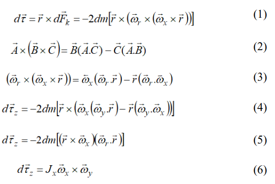
In more detail, this looks like this: We express the moment in terms of the Coriolis force. For any elementary mass dm with radius vector r and velocity v=ωr, the Coriolis force has the meaning (1). We apply the identity for a double vector product (2). For the inner bracket we obtain (3). Substituting back into (1) and obtaining (4). Since vector rxr=0, the second term disappears and remains (5). When integrating the entire mass volume of the disk, the terms containing r become the mass moment of inertia J. After transformations, we obtain (6). This shows that the total effect of all Coriolis forces is equivalent to the vector product of two angular velocities, scaled by the inertia of the body along the axis of rotation.

This explanation is by no means the only one circulating in the information space. Therefore, many readers will not agree with what is proposed here, because they probably have their own favorite explanations. On the Internet you can find several dozen videos, for example[1-3], where the secrets of the gyroscope are explained live. A good read is where 23 pages describe in detail various aspects of the gyroscope phenomenon [3]. In many other textbooks the explanations are reduced to the typical ones: “If a body rotates around X and turnes around Y, then it is quite natural for a torque to appear around Z, because that is what the vector product predicts”. Have you ever wondered why there are so many explanations for one phenomenon? Why, for example, is there not much discussion about the phenomenon of Newton’s Third Law Fa=Fr? Because it is exhaustive! Why do we continue to publish about the Gyroscope, including publications with such pretentious titles, although everyone claims that everything was discovered a long [4], long time ago? What is the problem? Probably the problem is in the approach. We accept Classical Mechanics as something monolithic that has long been completed in the most perfect way, and therefore there are simply no problems there. But this is not at all the case. There are many unsolved problems in Classical Physics:

• The Problem of the Inconsistency in the System of Newton's Laws: The First Law regulates conserved velocity and direction, but the Second and Third deal only with conserved velocity.

• The Problem of the Fictitious Force F=f(vω), according to which force can be created from conserved velocities. This is direct agitation for a Perpetual Motion! Incitement to a Perpetual Motion has been a punishable act in Classical Physics for centuries.

• The Cross Product τz=J_xω_xx_ωy. Should Not Be Possible because it connects mutually perpendicular vectors that Should Be Mutually Isolated according to the Principle of Galileo's Projections. The Gyroscopic Torque Phenomenon Should Not Physically Exist, nor the Cross Product. And if they do exist, then this means that there is something that Classical Mechanics misses.

• The problem is that the vector product τ_z=J_xω_xx_ωy does not correspond to the vector sum.

• The problem is the unidirectionality of the vector product J_xω_xx_ωy→τz [5].

• The vector product does not comply with the Superposition Principle.

• The idea of a Second Principal Motion in Classical Mechanics is not very good, because the vectors of the Second Principal Motion do not reflect all aspects of rotation.

• Why is the fundamental Inertia forming our fundamental idea of the material world considered fictitious, and is not part of the Fundamental Forces?

This is not all, but the Author suggests that this is enough for us to reach the conclusion that perhaps it is time to expand the framework left to us by the Fathers of Classical Mechanics. If we do not do this, then no matter how we twist and turn what is well established, we will get the same thing over and over again, or at most something similar to the same thing. For example, we can create a new mnemonic rule, such as the rule of two (appropriately oriented) crossed elbows. This will operate in parallel with the existing ones in Fig. 1. Thus we will claim great progress in development, and at the same time we will reinforce the existing approach, implying that nothing outside this (well-established) approach can be created. But mnemonics (memory aids) are based not on the physical nature of the phenomenon but on the symbolism of the phenomenon for the purpose of quick orientation. Therefore, a truly new approach can only be had if we abandon the idea of symbolizing and try to get down to the physical nature of inertia. Such an approach is no longer symbolic (mnemonic), but is truly physical (inertial). The fathers of Classical Mechanics did a remarkable job in those distant eras. Perhaps it's time for us to do something useful, in the modern 21st century.

New Method for Determining the Direction of Gyroscopic Torque

Nonlinear Dynamics

For more than twenty years the Author has been using in his theoretical and experimental works a New Method for Determining the Direction of the Gyroscopic Torque. It is a direct consequence of the wave nature of the formation of the gyroscopic torque, as described in [6,7]. The New Method is an application of the Second and Third Laws of Nonlinear Dynamics, see Figure. 3, which are developed in a series of three articles [8-10].

Figure 3: Laws of Linear and Nonlinear Dynamics

The need to add new laws to the three Newtonian ones arises from the fact of the so-called Inconsistency in Newtonian Laws. As revealed in, the Inconsistency consists in the fact that if Newton's First Law formulates two conserved potentials of inertial motion, velocity and direction, that is, velocity within the direction and direction within the velocity, then the Second and Third deal only with the inertial potential of the changed velocity within the direction. But what about the inertial potential of the changed direction within the velocity? As developed in Newton's First Law makes no distinction between the inertial potential of a changed velocity and the inertial potential of a changed direction. Both velocity and direction are conserved inertial states. Both are changed by an external force. Both inertial states resist the change with a force equal and opposite to that applied. What is the difference? The First Law makes no distinction [10,11].

As developed in the paragraph “About Mother Nature’s Rules” the inertial force of the changed direction is declared fictitious in Classical Mechanics [11]. The confusion comes from the fact that these types of forces and torques are functions of two velocities. Velocities in Classical Mechanics are conserved by virtue of the fundamental concept of Newton’s First Law, unlike acceleration. Conserved velocities are the basis of our well-established understanding of the physical world of inertia. Therefore, expressions such as and F_k=2mvω, F_c=mvω and τ_z=J_xω_xω_y show that something that changes inertia (force, torque) can be created from inertia that does not change (the product of conserved linear and angular velocities (vω)) [11]. And this is a direct request for a Perpetual Motion. To get out of this confusing situation, solutions are proposed. The well-established solution of Classical Physics is that F_k, F_c and τ_z are fictitious and therefore we do not need to deal with this. The solution proposed in [11] is that vω is not a product of two conserved velocities, but is a non-conservable complex velocity, also by Newton's First Law. We would find at least two differences in the chosen concepts:

First: The well-established Classical concept seeks solutions in Fk, Fc and τz, declaring these forces and torques to be fictitious. That is, the solution of Classical Physics is addressed to the left-hand sides of the problem equations F_k=2mvω, F_c=mvω and τ_z=J_xω_xω_y. In contrast, the concept of Nonlinear Dynamics from is to seek the solution in vω and ωxωy, that is, in the right-hand sides of Fk=2mvω, F_c=mvω and τ_z=J_xω_xωy [11].

Second: The solution of Classical Physics is addressed primarily to human activity “Don’t deal with this because F_k, F_c and τ_z are fictitious!” The solution from [11] is addressed to the physical nature of inertia: v and ω are conserved classical speeds but vω is non-conserved complex speed.

By the way, the Coriolis force F_k=2mvω is no less fictitious than the centrifugal force F_c=mvω, because both are based on the same inertial phenomenon (vω), (F=f(vω)). Despite its centuries-old development, Classical Mechanics has not yet developed an acceptable physical explanation of the phenomenon F=f(vω), as a counterpoint to F=ma. But nevertheless, it willingly uses the fictitious Coriolis force in the developments from (1) to (6) to explain the origin of the gyroscopic torque. However, when the same building “brick” (vω) is used to explain Reactionless Motion, then Classical Physics says: “This is impossible because F=mvω is fictitious, because it violates the “legal” F=ma”. Why does Classical Physics use a double standard?

Of course, if we do a historical review of the creation of the vector product we will get to the merits of William Hamilton, Josia Gibbs and others, who developed the ideas of dot product, cross product, vector multiplication and others. The story describes mathematician Sir William Rowan Hamilto’s discovery of quaternions on October 16, 1843, after years of trying to explain complex numbets of three dimentions, often asked by his childten if he could “multiply triplets” [12]. While walking along the Royal Chanel in Dublin, he realized the solution requared four dimentions, engraving the fundamental formula into the stone of Broom Bridge, where a commemorative plaque now stands. Hamilton’s work on quaternions directly led to modern vector calculus, including the vector product. The story is legendary. Although some versions refer to the “gyroscope puzzle” (since quaternions are now key to calculating the rotation of objects in 3D space), the original “childish” question was about multiplying triplets. Every year on October 16, mathematicians from around the world gather for the “Hamilton Walk” to honor that moment of genius.

One rational explanation is that the inertial phenomenon of the gyroscope was imposed on Classical Physics. Ceramic top-spindles were used as toys as early as ancient Egypt. Classical Physics cannot escape the “boxing ring” of the gyroscope by declaring “We don’t deal with that!”, as it does with the “boxing ring” of Reactionless Motion. It is forced to find a solution. Placed in a primary situation in which there is a phenomenon and no explanation, Physics usually first investigates the phenomenon experimentaly. Then it makes a breakthrough by constructing a scalar empirical relation τ_z=J_xω_xω_y. But this relation is scandalous because it connects perpendicular vectors that should be isolated according to the foundation of Classical Mechanics. We cannot multiply triplets. Then Physics looks for how to “dress” this scandalous empirical notion in a legitimate theoretical form. Of course, first solutions are sought with the existing vector sum. But it is obvious that it cannot be used, because no matter how much we sum ωx and ωy vectors, we will never get the perpendicular direction of τz. Then Classical Physics finds a solution in the rule of the vector product τz=Jxωxxωy, designed to legalize the impossible connection between three mutually perpendicular vectors. In this way, Classical Physics tells us: “Look, there is nothing scandalous in the fact that three mutually perpendicular (and isolated) vectors are connected, this is a completely normal connection”. This well-established attitude prevents us from realizing that by discovering the vector product we discover a model of a symbolized physical entity, and not the physical essence itself. If we had not found the vector product, then we would certainly have found another model. This is possible because the physical essence is one, and the models of the physical essence are infinitely many.

For example, in contrast to this, Reactionless Motion is not imposed on Classical Physics, and therefore it can declare “We are not boxing with this”. Reactionless Motion is a test of intelligence, how to build a new solution with the old “bricks”. Will we find an opportunity that is not forced upon us? By the way, there are other rules in life: If you consider yourself a champion, you must box with every contender. If you refuse to box, then you are no longer a champion. Perhaps we will look at the Laws of Nonlinear Dynamics not as some whim, but as a necessity. Perhaps we will look at them more seriously, as the only possible development originating from Newton’s First Law.

Second and Third Laws of Nonlinear Dynamics The Laws of Nonlinear Dynamics

are a consolidated expression of the inertial effect of the changed direction of a linear momentum mv with an angle α, see Fig. 4. Physically, the change in direction of one mv with an angle α occurs smoothly, along an arc 1-2-3. The elementary inertial forces of the changed direction, known as centrifugal forces, are distributed evenly along the arc. They look like a bent field of forces. This is the field of unconsolidated centrifugal forces, because their action is not consolidated in one direction, but is dispersed in many successively close directions. To establish the total inertial effect, we must consolidate the dispersed forces into a total magnitude acting along one total direction. This is what the Second and Third Laws of Nonlinear Dynamics do. In other words, the Laws of Nonlinear Dynamics transform the dissipated rotational energy of the changed direction into a consolidated translational momentum of the changed velocity by controlling (summing) the discrete dissipated portions.

Figure 4: Consolidated Inertial Effect of the Changed Direction of mv

It is obvious that the total magnitude (scalar) is equal to the vector sum of all elementary Fc=mvω. Since all Fc=mvω are equal in magnitude and differ only in direction, we can sum them with a simple integral [10,13]. It is even easier when we represent the consolidated magnitude as the vector sum of the momentum Ft created by the momentum of the input moment mv (Ft=mv) and the equal and opposite Ft of the output mv [8-10]. Thus, we replace the smooth diffuse release of Fc=mvω at a smooth change in angle α and v=cost, with a vector sum of the momentum Ft=-mv of a smooth decrease in velocity v to 0 at a constant direction from points 1 to 4, and the momentum Ft=mv of a smooth increase in velocity from 0 to v from points 4 to 3. Thus, we replace the diffuse effect of the fictitious Fc=mvω (when the velocity is constant, the direction changes) with a vector sum of two legal Ft=mv (the direction is constant, the velocity changes). In both cases, we obtain the same result: the magnitude (scalar) of the inertial potential predicted by Newton's First Law of the changed direction of one mv with angle α is equal to Ft=2mvsin(α/2). But as we have already said, if in the first case Ft is a vector sum of elementary fictitious Fc=mvω, and that's why Ft is fictitious, then in the second case Ft is equal to a vector sum of two macro “legal” Ft=mv from Newton’s Second Law, and that's why Ft is legal. That is, the derivation (formulation) by means of a macro-vector sum of two Ft=mv has the advantage of being derived directly from Newton’s Second Law. Moreover, a vector sum of two macro vectors is simpler than an integral. Thus, Ft=2mvsin(α/2) successfully unites the concept of centrifugal force Fc=mvω with linear momentum from Newton’s Second Law Ft=mv. Therefore, the Second Law of Nonlinear Dynamics for the consolidated inertial effect of the changed direction within the velocity appears as a reformulated Newton's Second Law for the inertial potential of the changed velocity within the direction.

The consolidation in Fig.4 establishes three important angles: This is the angle (α) of refraction (or bending) of the incoming and outgoing mv; this is the angle (π-α); and this is the angle (π). It is obvious that the direction of the consolidated Ft=2mvsin(α/2) passes through point 2 in the direction of the bisector of the angle (π-α) on the convex side of the refraction outward.

A New Method for Determining the Direction of the Gyroscopic Torque from the Point of View of the Laws of Nonlinear Dynamics

We come to the crux of this article: To determine the direction of the gyroscopic torque we simply need to apply the Laws of Nonlinear Dynamics of Figure. 4 to the gyroscope. We will use the theoretical statement for the Coriolis force of Figure. 2 unchanged. We agree that the points of application of the forces from the gyroscopic pair must be points A and B, both if the forces are Coriolis (Figure. 2) and if the forces are the result of an inertial effect of the changed direction (Figure. 4 and Figure. 5). But when the forces are the inertial effect of the changed direction of the orbital velocity in the X-Z plane (perpendicular to Y, Figure. 5), then points A and B are consolidation points equivalent to point 2 of Figure. 4. The directions of the peripheral velocities at points A and B in Figure. 5 are vertical as in Figure. 2. To adapt the directions of Figure. 5 to the theoretical setting of Figure. 4, we show the four possible cases of the Third Law of Nonlinear Dynamics vectors in Figure. 5a/. For our convenience, from now on we will write only v instead of mv, and only F instead of Ft. In all figures, the input velocities v (mv) are shown in blue and the output velocities v (mv) are in green. The generated forces F (Ft) and gyroscopic torques are in red.

We consider three steps:

First: Let the flywheel in Fig.5 b/, c/ and d/ rotate around X with angular velocity ωr (ωx) for example counterclockwise. The peripheral velocity of each particle of the flywheel in Fig.5 b/ will intersect the horizontal axis of turning (precession) Y from top to bottom at point A and from bottom to top at point B.

Second: Let the flywheel in Fig.5 c/ turns aroundYcounterclockwise with angular velocity ωt (ωy). Then the downward velocity coming out of point A will deviate (bend) to the right, as in case 1 of Fig.5 a/. The upward velocity coming out of point B will bend to the left, as in case 3 of Fig.5a/. Therefore, simultaneously with the turning of the flywheel around Y, we physically turn the velocities coming out of points A and B.

Third: The right-bent output velocity at point A will create a momentum F_t (denoted as F) directed to the left, Fig. 5 d/. The left-bent velocity at point B will create a momentum directed to the right. The two forces (impulses) act in opposite directions from diametrically opposed points with respect to Z, and create a torque τz directed clockwise.

Figure 5. Application of the Third Law of Nonlinear Dynamics to Determine the Direction of the Gyroscopic Torque. a/ Four Possible Cases in a Vertical Configuration. b/ Determination of the Directions of the Peripheral Velocities at Points A and B Intersecting the Axis of Turning Y. c/ Determination of the Directions of Refraction of the Peripheral Velocities with the plane of turning X-Z. d/ determination of the directions of Ft=2mvsin(α/2) and of the gyroscopic torque τz about Z.

Figure. 6 shows the four possible combinations of peripheral velocity directions and bending directions with respect to Y, as shown in Figure. 5 a/. We will simplify the method further if, instead of turning the flywheel physically about Y, we turn only the output velocity. Furthermore, we understand that to determine the direction of the torque it is sufficient to consider the bending of the peripheral velocity at only one point. We choose point A simply because it is closer.

The first column (Figure .6) shows the directions of the incoming velocities at point A, determined according to the direction of ω_r (ω_x). The second column shows the directions of refraction of the outgoing velocities according to the direction of ω_t (ω_y). The third column shows the forces (impulses) generated by the change in the direction of the orbital velocity in the plane of refraction and the direction of the gyroscopic torque τ_z that they create.

Figure 6: The Four Possibilities for Refraction of Peripheral Velocities

We will further simplify the application of the New Method by removing the coordinate system with its directed axes, (Figure.7). We no longer need to determine whether the coordinate system is left or right-handed. We do not need to apply the right-hand thumb rule to determine the directions of rotation ωx, turn ωy and torque τ_z.

We simply need to determine the direction of the peripheral velocity intersecting the axis of turning (Figure. 7 a/) at one of the two sides of the flywheel. We then need to determine how the turning of the flywheel about this axis distorts the output velocity, Figure. 7 b/. This determines the direction of the inertial force, Figure. 7 c/. We know that a mirror inertial force is created on the diametrically opposite side. The two forces form the axis around which they rotate the flywheel.

Figure 7: Simplified application of the new method. a/ We determine the direction of the peripheral velocity intersecting the axis of turn. b/ We determine the direction of the peripheral velocity deflection according to the direction of turn. c/ We determine the directions of the inertial deflection forces and the torque.

The New Method for Determining Direction is Part of the Theoretical Formulation for Deriving the New Formula for the Gyroscopic Torque

The idea is to show that the New Method for Determining the Direction of the Gyroscopic Torque is not an isolated mnemonic (symbolic) rule, but is the theoretical formulation of the New Method for Determining the Gyroscopic Torque, developed in three papers [8-10]. Moreover, it is a small part of Nonlinear Dynamics.

Geometry of forces.

                                 Figure 8: Geometry of Forces and Torques

The forces of the gyroscopic pair are created by the inertia of the mass. To create a unidirectional torque, the forces must act in opposite directions with respect to Z, Figure. 8. But the masses rotate about X and therefore they periodically change their position with respect to Z. Respectively, each mass changes its position from point A to point B and vice versa. Therefore, a unidirectional torque can be created only if the masses change the directions of the inertial forces that they create simultaneously with changing their positions. The gyroscopic forces creating a unidirectional torque must be periodically alternating in sign. This issue is developed in more detail in [6] and especially in [7]. It is stated there that even if we do not know what the physical origin of the forces (Coriolis or other), they must certainly be alternating in order to create a unidirectional torque.

If the force created by a mass is in opposite directions at points A and B, then this means that when moving from A to B, the force smoothly changes direction from +1 to -1 and vice versa. This means that the transition from +1 to -1 and vice versa passes through 0. Therefore, the mass (sector) should not create a force when passing through the intermediate points C and D. Therefore, the force is maximum but in opposite directions at A and B, but it is equal to zero at C and D. That is, the torque created by two diametrically opposed masses is pulsating: it is maximum when the masses pass through points A and B, but is equal to zero when the masses pass through points C and D.

This gives us reason to call the line connecting the consolidation points A and B “Maximal Magnitude line” because the masses create maximum forces and torque when they cross the points of this line. We call the line connecting C and B “Zero Magnitude&Inversion line” because the forces there are zero when they change their directions. It is obvious that the frequency of change of the gyroscopic torque is twice the frequency of change of the forces.

Speed Geometry

The velocity of any elementary mass or sector of the flywheel periodically undergoes two types of changes, Figure 9:

                                              Figure 9: Speed Geometry

First: When the mass passes through the Maximal Magnitude line its velocity is maximally refracted. If at point A the velocity bends to the right, then at B it bends to the left.

Second: When the mass passes through the Zero Magnitude&Inversion line, the peripheral velocity of rotation around X is not refracted, but instead is vectorially summed with the peripheral velocity of turning around v=vx+vy=R(ωx+ωy). If at point C the vector sum is directed to the left, then at D the vector sum is directed to the right.

The period of both types of changes is 2π. But they are phase shifted relative to each other by an angle π/2. The refraction is zero at points C and D where the vector sum is maximal, and it is maximal at points A and B where the vector sum is zero. Let us follow this in more detail, Figure. 9:

• from A to D the refraction to the right decreases and goes into an increasing vector sum to the right,

• from D to B the vector sum decreases and goes into an increasing refraction to the right,

• from B to C the refraction decreases and goes into an increasing vector sum to the left,

• -and from C to A the vector sum decreases and goes into a refraction to the right.

Coincidence

We can easily establish in Fig.9 that where the forces are maximum at points A and B where the refraction of the peripheral velocities is maximum. The forces creating the gyroscopic torque are zero where the refraction of the peripheral velocities is zero. This coincidence, accidental or not, represents the theoretical setting for deriving the New Formula, as well as for the New Method for determining the direction of the gyroscopic torque.

The New Method for Determining Direction is Part of the Theoretical Framework for Deriving the New Formula for the Gyroscopic Torque

The New Method for Determining the Direction of the Gyroscopic Torque exactly repeats the theoretical formulation used to derive the New formula for the gyroscopic torque from [8], [9] and [10]. Just as in Fig. 4 Ft=2mvsin(α/2) is collected (consolidated) at point 2 of the arc 1-2-3, so in Fig. 5 and Fig. 10 Ft=2mvsin(α/2) is consolidated at points A and B of the arcs C-A-D and D-B-A in the plane of turning about Y. Therefore, each π-rotation (arc) of an elementary mass from the flywheel from C to D and from D to C produces one Ft=2mvsin(α/2) applied at points A or B in the X-Z plane. We will not write the elementary mass as dm because it can be quite large, for example an angular sector of the flywheel.

Figure 10: Laws of Linear and Nonlinear Dynamics

In Figure. 10 we show the motion separately in the mutually perpendicular planes Y-Z and X-Z. In this way we isolate the velocities and centrifugal forces of the rotation about X from those of the turning about Y. The arcs C-A-D and D-B-C in the Y-Z plane form a closed trajectory because they are connected. Therefore, the centrifugal forces in Y-Z plane are mutually balanced. But the projections of the 3D arcs C-A-D and D-B-C represent open 2D trajectories C_{on leaving}-A-D_arriving and D_{on leaving}-B-C_arriving in the X-Z plane of the turning about Y. These open arc trajectories resemble the arc 1-2-3 in Fig. 4, so we apply the Laws of Nonlinear Dynamics as we did in Fig. 4. The Second Law of Nonlinear Dynamics sums up all the dissipated inertial forces of the changed direction along Con leaving-A-Darriving and Don leaving-B-Carriving and consolidates them into impulses Ft=2mvsin(α/2) applied at the consolidation points A and B. The impulses Ft=2mvsin(α/2) are radial to the turning of the masses of the disk along the arcs C on leaving -A-D arriving and Don leaving-B-Carriving and are consolidated at the points A and B. Therefore Ft=2mvsin(α/2) lie in the X-Z plane of turning about Y, and therefore they are perpendicular to the Y-Z plane of rotation of the disk.

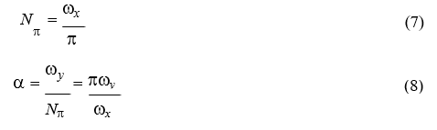
The Laws of Nonlinear Dynamics have given us the magnitude and directions of the gyroscopic forces without having to resort to the services of vector multiplication. Then we only need to calculate the magnitude of one consolidated impulse Ft=2mvsin(α/2), multiply the result by the number of impulses per second, and of course by the radius R, to obtain the magnitude and direction of the gyroscopic torque. To calculate single Ft=2mvsin(α/2) we need to know the orbital velocity v, and the angle α of turning (precession) of the flywheel about Y for each arc Con leaving-A-D_arriving and D_{on leaving}-B-C_arriving. To calculate the angle α we first need to calculate the number Nπ of π-arcs per second (7). Then we divide the angular velocity of turning (precession) about Y by Nπ and we obtain the angle α of turning for each arc C_{on leaving}-A-D_arriving and D_{on leaving}-B-C_arriving (8). Then (9) calculates the magnitude of one Ft=2mvsin(α/2) for one arc (one π-quantum). To determine the magnitude of the generated momentum Ft for one second we multiply both sides of equation (8) by the number Nπ of π-arcs Con leaving-A-Darriving and Don leaving-B-Carriving per second. We determine the torque about Z by multiplying both sides by the radius R (10). Then substitute in (11) v=ωxR. We integrate over the entire volume of the disk mass and obtain the mass moment of inertia J (J=mR2).We obtain the final equation for the generated gyroscopic torque (12),

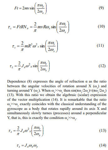
It turns out that in (14) we obtained the scalar form of the cross product of (6) as algebraic expression without using vectors and cross products to determine the direction of the gyroscopic torque. We do not need the right-hand finger rule to determine the direction of the given vector. We do not need the three-finger rule, nor the right-centered coordinate system, nor Rezal's theorem. We do not need Zhukovsky's rule, the pursuit rule, the active torque rule, multiplying triplets, the 90-degree rule, the dot product, the cross product, the quaternions, the complex analyses from (1) to (6) and so on. Instead of using all these mnemonic (symbolic) rules and conventions, we obtained the gyroscopic forces perpendicular to the plane of the disk as radial to the turning around Y (X-Z plane), applied at the consolidation points A and B. The work of determining the direction was done by the Laws of Nonlinear Dynamics.

The reader has probably noticed that the arcs C_{on leaving}-A-D_arriving and D_{on leaving}-B-C_arriving in Fig. 10 are not uniform, as are the arcs in Figure. 4. In addition, the orbital velocities at the points C_{on leaving}, D_arriving, D_{on leaving} and C_arriving are perpendicular to the X-Z plane. In order to determine the consolidated Ft=2mvsin(α/2) in non- uniform arcs, we have developed and applied theorems. There are three groups of 2D theorems:

• The first group of 2D theorems regulates the consolidated Ft=2mvsin(α/2) in non-uniform but symmetric arcs such as C_{on leaving}-A-D_arriving and D_{on leaving}-B-C_arriving.

• The second group of 2D theorems regulates the consolidated Ft=2mvsin(α/2) produced by arcs on which radial and tangential accelerations act simultaneously. That is, this is the case when the mass simultaneously changes direction and speed. • The third group regulates the peculiarities of the periodicity of Ft=2mvsin(α/2). In addition, it is clear that we have the tools to consolidate the inertial effects of changed speed and changed direction both separately and together not only along the symmetric line 2-4 of Figure. 4. but also along any other radial line of the arc.

There are also 3D theorems that regulate the specifics of motion along complex 3D arcs. We will not develop these theorems here because we will need 80-100 pages. Now it is important for us to know that the consolidated Ft=2mvsin(α/2) created by the uneven but symmetric 2D arcs of Figure 10 is no different from the Ft=2mvsin(α/2) created by the even arcs 1-2-3 of Figure 4. In other words, we can look at the uneven but symmetric C -A- _arriving and D_{on leaving} B-C_arriving in the same way as we look at the arc 1-2-3 of Figure 4.

Analyses, Comparisons, Theses, Perspectives

At first glance, the following goes far beyond the initial idea of announcing the New Method for Determining the Direction of Gyroscopic Torque. The purpose of this part is to show that the Old Vision of the Gyro, although well-established, suffers from serious fundamental flaws, because it was created in Violation of Basic Rules. For these reasons, it is not capable of creating further developments, and therefore it is a vision without perspective. Yes, the Old Vision gives us a working formula to determine τz and rules to determine its direction in a particular case ωx>>ωy. This gives us the opportunity to use the gyroscope in inertial navigation, in the particular case of Control Moment Gyros, as a sensor in electronics, but that's all.

The idea is to show through analyses and comparisons that when creating the New Vision, the fundamental flaws of Violation of Basic Rules have been avoided. This gives the capacity to generate developments in the direction of Nonlinear Dynamics. Nonlinear Dynamics is huge. Here we have selected a compilation of just 20 points, presented in the shortest possible way. It is assumed that they can paint the big picture. The reader who has never dealt with this will accept many of the presented theses as pure speculation.

1. The vector product used by Classical Mechanics to derive τ_z=J_xω_xx_ωy is pseudoscientific because it does not correspond to the vector sum. Mathematics is built on simple rules according to which any higher mathematical (algebraic) operation should be able to be represented by the lower one, because the higher one is a development of the lower one. For example, 3.5 is just a shortened notation of 3+3+3+3+3 or 5+5+5. If a vector product cannot be represented by vector sums, this means that it does not correspond to the vector sum, and therefore it is pseudoscientific. Another point is the lack well established understanding of the nessary vector division.

2.The algebraic (scalar) expression τz =Jx ωx ωy from (14) is completely sufficient to determine the direction of τz , because it defines the forces perpendicular to the disk of the gyroscopic pair as radial to the turning in the perpendicular plane.

3. The Laws of Nonlinear Dynamics provide a well-developed correspondence network between Newton's First Law, the Second Law F=ma (Ft=mv), F_c =mvω, Ft=2mvsin(α/2), τ_z =(2/π) Jx ω2 sin(πωy /2ωx ) and τ_z =J_x ω_x x_ωy .

4. The vector product τ_z =J_x ω_x x_ωy obtained in (6) cannot be decomposed back to the Coriolis force, because vector division is missing. The algebraic expression τz =J_x ω_x ω_y obtained in (14) by vector sums can be decomposed mathematically back to the centrifugal force.

5. The algebraic (scalar) form of the vector product τ_z =J_x ω_x ω_y is a special case of τ_z =(2/π)J_x ω₂ sin(πω_y /2ω_x ). That is, τ_z =(2/π) J_x ω2 sin(πωy /2ωx ) is the big one and τ_z =Jx ωx ωy is the small one. Therefore, τ_z =(2/π)J_x ω₂ sin(πωy /2ωx ) is not only τz =Jx ωx ωy , but it is also something much more.

6. The geometry of the gyroscope is such that only a sign-changing force created by a mass dm can create a unidirectional torque. Therefore, the Coriolis force must act as +F and –F for periods Δt, that is, through impulses +Ft and -Ft. The classical derivation by the double vector product of (1) to (6) ignores this, as well as the fact that the Coriolis force acts scattered along a π-arc (similar to the centrifugal force in Fig. 4) and therefore its action must be summed (consolidated) over the entire arc at the point of application. The classical derivation “skips” all this. It simply takes Fk =2mvω at the point of application, and then calculates the macro result τ_z =J_x ω_x xωy . In contrast, Nonlinear Dynamics creates the function F_t=2mvsin(α/2) by a vector sum of elementary F_c =mvω. In turn, the function, τ_z =(2/π)J_x ω2 sin(πωy /2ω_x ) is created by sums of unit portions (quanta) of F_t=2mvsin(α/2). Therefore, the derivation of τz consists only of a series of vector sums and is therefore “legal”. The vector sum restores the connection between the “low rank” of the sum and the “high rank” of the torque τz , which is Violated in the vector product. The method through vector sums does not rely on the “magic” appearance of the perpendicular vector at the expense of the vector product rule, but builds it step by step by summing the impulses. Therefore, it is mathematically more robust for describing the wave and periodic nature of the gyroscope. Nonlinear Dynamics is “transparent”.

By “skipping” the vector sum of the impulses +Ft and –Ft in the formation of a unidirectional gyroscopic torque, the Classical derivation ignores the periodicity of opposite phase states of inertia, although it assumes that they form τ_z =J_x ω_x x_ωy . Thus, the role of the dynamic phase states remains hidden and the macro result is given directly. In this way, Classical Mechanics blinds itself and remains without a sense (instrument) for these phase states.

8. This turns out to be a critical flaw in order to understand that if for any elementary mass Ft are sign-changing and τ_z is pulsating, then this means that the forces pass periodically from +Ft to –Ft and then to +Ft, through zero values, although all the time v≠0 and ω≠0 (see Fig.8 and 9). Therefore, there are three phase states: +F, –F and 0. We encounter an inertial phenomenon “Zero Force” in which the force Fc =mvω=0 or Fk =2mvω=0, although m>0, v≠0 and ω≠0. In fact, if there are movements (energy) at the zero points but no gyroscopic forces, this means that the inertia creating the gyroscopic torque is "off" or "zeroed". Later we will call this phenomenon “Inertia Valve”.

9. Classical Mechanics does not accept this because it considers inertial interactions only in the conditions of an analog continuum where no one can “turn off” inertia. We identify inertia only through the inertial force of a mass when it changes speed or direction. Therefore, when we say that no one can “turn off” inertia, we mean that no one can turn off the inertial force in the analog continuum. That is, if a mass m>0 is accelerated with a≠0 in the analog continuum, then always F=ma ≠0, and no one can make even for an instant F=ma=0 when m>0 and a≠0. Also, no one can make F_c =mvω=0 or F_k =2mvω=0 when m>0, v≠0 and ω≠0.

Classical Mechanics accepts that it is possible Fc =mvω=0 in the inflexion of a change in curvature because there ω=0. But the geometry of the gyroscope offers a case in which the velocities at the inflection points C and D are non-zero (v≠0 and ω≠0), and yet F_c =mvω=0 (F_k =2mvω=0). In Algebra there is a Zero Product Law, according to which a product is equal to zero if and only if at least one of its factors is equal to zero. But obviously our case is not like that because the force is equal to zero even though all three factors are non-zero. Of course, Classical Mechanics has found a solution: in fact, the factors are not three but four. The fourth factor is the sine of the angle between v and ω. Since at the zero points C and D of Fig. 2 the vectors are collinear, then sin(0)=0 and then Fk =2mvωsin(0)=0. Okay, but if the actual formula is not Fk =2mvω, but Fk =2mvωsin(φ), then why is it not involved in the classical derivation from (1) to (6)? Why was the periodic Fk =2mvωsin(φ) not taken instead of the analog Fk =2mvω? If at the zero points C and D Fk =2mvωsin(φ)=0 and at the applied points A and B Fk =2mvωsin(φ)= 2mvω because sin(π/2)=1, then what is Fk =2mvωsin(φ) at all other points on the arcs C-A-D and D-B-C? Why is it that when we talk about Fk =2mvω=0 at the zero points we think of the fourth term sin(φ), but for all other points on the arcs it does not exist? Yes, such are the rules of the vector product. These rules are mnemonic, detached from physical reality they are designed to explain.

10. These are theoretical disputes. The important thing to understand is that regardless of the outcome of the argument, the force F=mf(vω)=0 is indeed true regardless of m>0. v≠0 and ω≠0 at the inflection (zero) points C and D. It is important to understand that theoretical argument cannot change the physical phenomenon. Discrete Nonlinear Dynamics accepts the physical fact that for this short phase Δt of the cycle the force F=mvω=0, even though m>0, v≠0 and ω≠0. Classical Physics excludes the possibility of such a development. It calls this a “Violation of Well-Established Natural Laws” and Punishes Violators.

11. Ignoring the cyclic wave character and calculating the result directly, Classical Physics accepts as “legal” only phase states +F and –F. Therefore, it calculates only symmetric cycles of the type +F, –F, +F, –F, which we write as +1, -1, +1, -1. Classical Mechanics skips the zero between +1 and -1 and states “Here, only +1, -1 cycles can exist. Nobody can accumulate a one-way inertial potential because nobody can “turn off” inertia, that is, the inertial force. And if someone does this, it will be a “Violation of WellEstablished Natural Laws”.

12. Nonlinear Dynamics includes the phase with the “turn off” of the inertial force and defines three phases: +1, 0 and -1, instead of two +1 and -1. Therefore, it defines the cycles as +1, 0, -1, 0, +1, 0, -1, 0, +1, see Fig. 8 and 9. From here on, Nonlinear Dynamics can do anything: It can also construct a symmetric phase cycle +1, -1, +1, -1 and prove that no one-way inertial potential can be accumulated. What's more, if you want to delve into this, you will notice that a cycle +1, 0, -1, 0, +1 contains two zeros. We can write the phases as follows: +1, -0, -1, +0, +1. Here -0 is the phase at the transition from +1 to -1, and +0 is the phase at the transition from -1 to +1. Therefore, we now have four phases: +1, -1, +0 and -0. Then Nonlinear Dynamics can compose a new symmetrical cycle of phases -0, +0, -0, +0, and again prove that a unidirectional inertial potential cannot be accumulated. But Nonlinear Dynamics can compose asymmetrical cycles of phases +1, 0, +1, 0 or -1, 0, -1, 0 to prove that a unidirectional inertial potential can be accumulated. Moreover, a test device can change the phases in motion, such as: +0, -0, +0, -0, +1, 0, +1, 0, +1, 0, -1, +1, -1, +1, +0, -0, +0, -0, -1, 0, -1, 0, demonstrating different representations and abrupt changes.

13. In Classical Mechanics, the functions Fk =2mvω and Fc =mvω are analog. Expectedly τz =Jx ωx xωy is also analog, because it is derived from Fk =2mvω. But in Nonlinear Dynamics the analog Fc =mvω is transformed into the periodic (wave) function Ft=2mvsin(α/2), which is intrinsic to the logic of its derivation. Therefore, the application of Ft=2mvsin(α/2) leads to a periodic dependence τz =(2/π)Jx ω2 sin(πωy /2ωx ). It is always better to analyze the periodic change in the direction and magnitude of the forces from the gyroscopic pair with periodic functions, instead of analog ones.

14. Mechanics that is based on the periodicity of different phase states, which are exposed by deriving the algebraic τ_z =J_x ω_x ω_y through a double vector sum, is already periodic, cyclic, wave, discrete, digital and quantum. In this wave Nonlinear Dynamics the transition from the analog Fc =mvω to the wave Ft=2mvsin(α/2) is commensurate with the transformation of the analog F=ma to the wave F_t=mv, the right-hand side of which is multiplied by the wave operator 2sin(α/2). This is done by replacing the argument v of the analog Ft=mv with the argument α of the wave Ft=2mvsin(α/2). Then the analog τ_z =J_x ω_x ω_y is only a special case of the wave τ_z =(2/π)J_x ω² sin(πωy /2ωx ). Classical Physics does not offer a transition from analog τ_z to wave τ_z . It remains analog, closed in the analog continuum, and therefore it considers inertia only as analog.

15. The periodic relation τ_z =(2/π)Jx ω² sin(πωy /2ωx ) between vectors of X, Y and Z shows that the degrees of freedom are not connected “just like that”, because “just like that” they are isolated. Isolated analog vectors are connected periodically, wave-like, discrete, digital, quantum under given conditions, which are the subject of study by Nonlinear Dynamics. This simultaneous isolation “just like that” and connection under given conditions creates Inertial Indeterminacy (often used term singularity). Later we will put this Inertial Indeterminacy to work in the homogeneous space-time of Emmy Noether.

16. The discovery that the relation between the degrees of freedom is not “just like that” but is periodic, wave-like, discrete, digital, quantum gives us the opportunity to build new artificial relations, similar to the classical τ_z =J_x ω_x x_ωy . A total of eight such relations have been discovered so far. They are formulated as Nonlinear Inertial Protocols (NIP). By the way, the full name is “Nonlinear Protocols of Local Inertial Connection of Isolated Vectors in Homogeneous Spacetime”.

17. The vector sum is a direct consequence of the Galilean Projection Principle, which isolates perpendicular directions. Therefore, the vector sum, based on the cosine function, also isolates perpendicular vectors (directions). But in the developments (7) – (14) the double application of the same vector sum that isolates, leads to the expressions τ_z =(2/π)J_x ω² sin(πωy /2ωx ) and τ_z =J_x ω_x ω_y which do not isolate, but on the contrary, connect perpendicular vectors. Of course, perpendicular vectors cannot be connected “just like that”, because no matter how much we sum “just like that” the vectors ωx and ωy we will never get the perpendicular direction of τ_z . It turns out that we need to know what and how to sum. It also turns out that using vector sum correctly we can get antagonistically contradictory results: from isolated by vector sum perpendicular vectors to connected by vector sums perpendicular vectors. Further, encountering this contradiction in different Nonlinear Inertial Protocols again and again, we will be forced to formulate “Uncertainty in Nonlinear Dynamics”.

18. Noether’s theorems are a continuation of the classical idea that the Universe is an analog continuum. They assume that an analog homogeneous spacetime is neutral to mass (inertia) and therefore cannot create Reactionless Motion. Only an inhomogeneous spacetime can change the state of mass, and this is probably the case. Analog Newtonian and Classical Mechanics predict that Reactionless Motion is possible only if F1 =F2 is Violated, and this is a Perpetual Motion. Thermodynamics supports that Reactionless Motion is a Perpetual Motion of the First, Second or Third Kind. But neither the analog homogeneous continuum of Noether, nor the analog linear Newtonian and Classical mechanics, nor Thermodynamics allow that such a spatial wave inertial relation is possible in which periodically for short Δt perpendicular vectors can be connected to create a mutually perpendicular product, nor that berween these periods there are other periods (points) where the force Fc =mvω=0 in the plane of rotation, although m>0, v≠0 and ω≠0. Therefore, they do not foresee cycles: +1, 0, +1, 0 or -1, 0, -1, 0.

19. The solution τ_z =J_x ω_x x_ωy derived from a higher rank vector operation (product) is an exhaustion of higher possibilities. When a vector product does not correspond to a vector sum, it offers false possibilities. The solution τ_z =J_x ω_x ω_y derived from a lower rank vector summation represents the discovery of new possibilities. If the cross product solves a problem that can be solved by a vector sum, this is not good for the system, even if the cross product is not pseudoscientific because it corresponds to the vector sum. For a hierarchical system, it is always better to solve problems from a lower rank rather than from a higher one, because this does not exhaust the capacity of the higher rank.

20. The principle of Occam's Razor predicts that when there are many explanations for a phenomenon, then the simplest one is the most correct. Comparing the double application of a simple sum with the double application of a complex cross product, even if we do not take into account that the cross product is pseudoscientific, we will find that Occam's Razor mercilessly cuts out the complex Classical cross product τz =J_x ω_x x_ωy (6), and remains the simple double vector sum, which we write for short as τ_z =J_x ω_x ω_y (14).

Some Brief Summaries, Discusions

Classical Physics is a science of equilibrium and average values of the final result. It is not interested in the phases through which one passes to obtain the result. Instead, it is only interested in the final result, because it believes that whatever the phases are, the final result is always the same. This is clearly seen from the nature of Rezal's theorem, the rules of pursuit, Zhukovsky's, Foucault's, the vector product's, 90-degree rule, the right screw's, the three fingers' and so on, all of which are focused on the final result. This is seen from the classical derivation of the vector product from (1) to (6): it avoids the detail of the vector sum, the element and the phases and gives the final result directly. This is seen from the sources, all of which are focused on the final result [1-3]. The "smooth" averaged motion is preferred because it is easier to calculate. The zero point of inertial force is considered a mathematical curiosity, not a working resource. The zero point means that the machine must be nonlinear and non-stationary. Classical Physics of equilibrium and average values avoids technological difficulty because it is designed to design and operate stable, predictable and symmetrical machines. At present, if someone says “I will use the zero point to create Reactionless Motion”, he will be automatically classified by the scientific community as a seeker of Perpetuum Mobile. Although on the one hand Cassical Physics actively promotes the Perpetual Motion using forces or torques that are a function of the product of two conserved velocities, on the other hand it actively fights against the Perpetual Motion. Classical Physics, which does not notice and does not resolve this (and other) contradictions, cannot create anything more complex than a analog rocket engine operating in a homogeneous space with isolated degrees of freedom.

The truth is that the related degrees of freedom, the zero point, the heavy mass, the uncertainty, etc. cannot exist if they violate the Laws of Physics. Yes, they may violate Well-Established Human Concepts of Physical Laws, but they cannot violate the Laws of Physics. It is the height of complacency and arrogance to assume that Well-Established Human Concepts are identical to Physical Laws, or that we will determine Physical Laws, especially using the Well-Established “highly productive” and “scientific” method of not bothering with this. Obviously we do not understand that Human Concepts change but Physical Phenomena remain. Therefore, Nonlinear Dynamics focuses on the detail. For example, if the Classical concept determines the direction of the gyroscopic torque through the final result, then the New method does this through the detail of the momentum Ft. A detailed consideration of the inertial interaction (instead of the generalized, averaged values) reveals the detail, the element, the phase, the zero point, the uncertainty, the velocity resistance and many other “trifles”. Further, these “insignificant trifles” can be used to create unconventional inertial interactions in a Nonlinear Wave Dynamics.

Conclusion

The forces of the gyroscopic pair are perpendicular to the plane of rotation of the disk, because they are radial to the turning in the perpendicular plane of rotation (precession).

It is amazing to note that this simple vision has remained hidden from Well-Established Classical Physics throughout all the long centuries of “Well-Established”. Therefore the argument “We do not concern ourselves with this because it is Well-Established that it is Impossible” is dethroned. Classical Physics which prefers the complex to the simple, which uses pseudo-scientific vector products and fictitious forces instead of vector sums, which calls the zero point of the periodic change of +F to –F a Violation, cannot consider itself “Well-Established”. It seems that we have not learned our historical lesson and have rushed again with Violations and Punishments, just like four centuries ago. But of course, we cannot know this because we do not concern ourselves with it.

Declarations

Funding: This research received no specific grant from any funding agency.

Conflict of Interest: The author declare no conflict of interest.

Author Contributions: Djordjev, Bojidar.

AI Usage Statement: AI tools were not used at all.

References

1. Online video, Physics Unsimplified, The mystery of gyroscopic motion: How Does it Do That?
2. Online video, Michael van Biezen Physics 13.6 The Gyroscope (3 of 5) The Torque of Spinning Gyroscope.
3. OpenCourseWare, M. I. T. Free Onliine Course Materials, Classical Mechanics, Online Textbook, Chapter 22 Three Dimensional Rotations and Gyroscopes.
4. Usubamatov, R., Harun, A.B., Fidzwan M., Md. Hamzas, A. (2014). Gyroscope Mystery is Solved. International Journalof Advances in Mechanical and Automobile Engg. (IJAMAE) Vol.1, Issue1 (2014) ISSN 2349-1485 EISSN 2349-1403.
5. Djordjev, B. (2024) One Way Equations in the Classical Mechanics. Conservation Laws. Preprint
6. Djordjev, B. (2008). Free (Reactionless) Totque Generation Fiction or Reality, CONTROL'08: Proceedings of the 4th WSEAS/IASME international Conference on Dynamical Systems and Control
7. Djordjev, B. (2010). Free (Reactionless) Torque Generation—Or Free Propulsion Concept, Publication date 2010/1/28, Journal AIP Conference Proceedings, Volume 1208, Issue 1, Pages 324-338, Publisher American Institute of Physics.
8. Djordjev, B. (2014). New method to explain and calculate the gyroscopic torque and its possible relation to the spin of electron, Volume 1, Issue ISBN: 978-960-474-377-3, Pages 55-62ctron. 10th International Conference on APPLIED and THEORETICAL MECHANICS (MECHANICS '14)
9. Djordjev, B. (2014). New Formula to calculate the gyroscopic torque and its relation to the spin of electron, Conference SCIENTIFIC PROCEEDINGS XXII INTERNATIONALSCIENTIFIC-TECHNICAL       CONFERENCE      "trans      & MOTAUTO ’14", Volume 2, Issue ISSN 1310-3946, Pages31-34
10. Djordjev, B. (2014). Reactionless motion explained by the Laws of the Nonlinear Dynamics leading to a new method to explain and calculate the gyroscopic torque and its possible relation to the spin of electron, WSEAS TRANSACTIONS on APPLIED and THEORETICAL MECHANICS.
11. Djordjev, B. (2025). Step derivative equations of inertial motion in the Classical Mechanics. Conservation Laws, Journal International Journal of Physical Sciences and Research, Volume 1, Issue 1, Publisher International Glint Publications
12. Wikipedia, Free encyclopedia, History of Quaternions.
13. Chu,  W.,  Mayer,  J.W.,  and.  Nicolet,  M-A.  (1978).Backscattering Spectrometry, Academic Press, page 23.
14. Djordjev, B. (2025). Acceleration-Acceleration, Acceleration-Velocity, and Four More Modes of Application of Newton's