A New Classical Physics Theory Applicable to Objects Moving at High Speeds

Introduction

Newton’s “The Mathematical Principles of Natural Philosophy” laid the theoretical foundation for classical physics. Nevertheless, in this seminal work, Newton did not introduce the concept of a finite propagation speed for forces. Instead, scientists at the time universally assumed that force transmission was instantaneous, that is, its propagation speed was considered infinite. Consequently, the mathematical formulations of Newtonian mechanics do not include any physical quantity representing the speed at which forces are transmitted [1].

Currently, scientists have established that the four fundamental interactions in nature are mediated by fields that propagate at the speed of light [3,4]. This observation raises an important question: Does the finite propagation speed of forces affect their magnitude? The answer is affirmative. In the following section, the impact of the finite speed of light on time is first examined.

Effects of the Finite Speed of Light on Time

As shown in schematic diagram 1, consider two particles, Z1 and Z2, in space. Particle Z1 is located at the coordinate origin, whereas particle Z2 is positioned at the coordinate M₁. Both Z1 and Z2 are equipped with an identical clock, and the readings on both clocks are always synchronized. At time T = 0, two spherical light waves, Q1 and Q2, are successively emitted from particle Z1 at a time interval of τ, with the light propagating at a speed of C.

Temporal Variations for Particles at Relative Rest

When particle Z2 remains stationary at coordinate M1, calculations indicate that the time interval t0 displayed on the clock of particle Z2 between the receptions of spherical light waves Q1 and Q2 is equal to the emission time interval τ, that is,

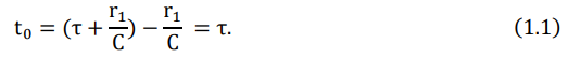
Here, t₀ is defined as the static time interval.

Temporal Variations for Particles in Relative Motion

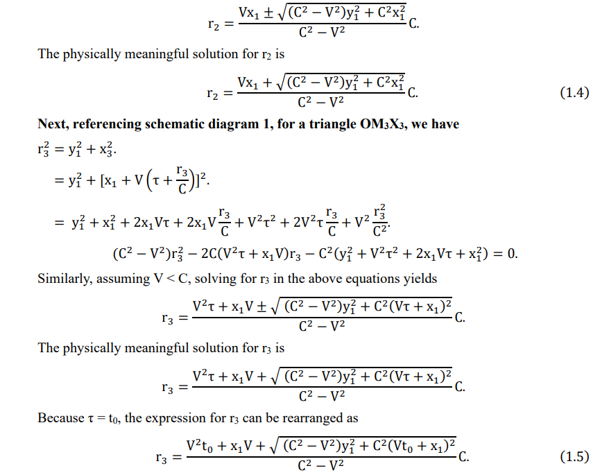
At time T = 0, simultaneously with the emission of the first spherical light wave Q1, particle Z2 commences uniform rectilinear motion from coordinate M1 along the positive X-axis at a constant speed V. This particle subsequently encounters spherical light wave Q1 at coordinate M2 and spherical light wave Q2 at coordinate M₃. Calculations reveal that when particle Z2 is in motion, the time interval t displayed on its clock between the receptions of spherical light waves Q1 and Q2 is related to the emission time interval τ by the expression

Here, t is defined as the dynamic time interval.

Functional Relationship Between Static and Dynamic Time Intervals

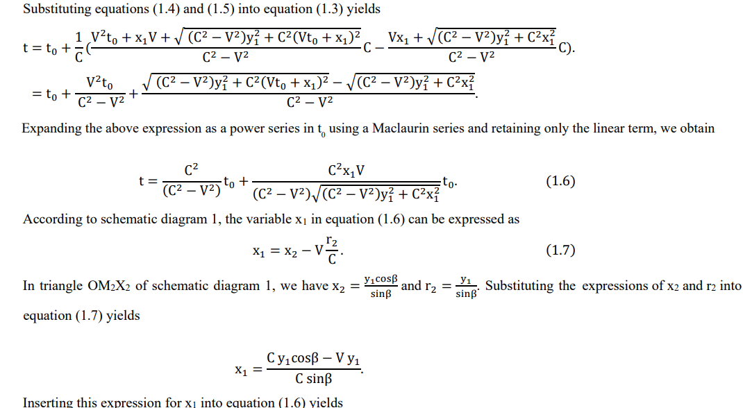
Because the static time interval t0 is always equal to the time interval τ between the emissions of the spherical light waves Q1 and Q2, substituting τ = t₀ into equation (1.2) yields

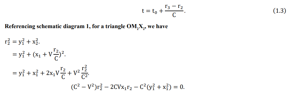
Assuming V < C, solving for r₂ in the above equations yields

 

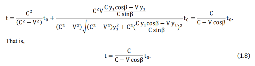
In equation (1.8), t represents the dynamic time interval between the two particles, t₀ denotes the static time interval, V is the relative speed between particles Z2 and Z1, β refers to the angle between the line connecting particles Z2 and Z1 and the relative velocity V, and C is the propagation speed of the light waves.

Equation (1.8) provides the functional relationship between the static time interval t0 when the two particles are at relative rest and the dynamic time interval t when the two particles are in relative motion. Equation (1.8) indicates that when the speed of light is infinite (C→∞) or when the relative velocity between the two particles is zero (V = 0), t is identical to t₀. Conversely, when C is finite and both V and cosβ are nonzero, t differs from t₀. Additionally, the ratio between these intervals varies as a function of the relative speed V. Therefore, the speed of light being finite is considered a necessary condition for the emergence of relativistic variations in time.

Relationship Between Static and Dynamic Time Intervals and The Doppler Effect of Light Waves

In theory, equation (1.8) can be directly applied to calculating the Doppler effect for light waves. As an example, consider a stationary light source emitting a series of light waves with a period T₀, where T₀ is equal to the static time interval t₀. When an observer moves in a uniform rectilinear motion relative to the light source at speed V, the functional relationship between the observed period T and the emission period T₀, according to equation (1.8), is given by

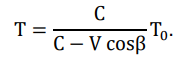
Based on this, the functional relationship between the emitted frequency f₀ and received frequency f is given by [3]

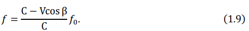
Here, f is the frequency of the light waves received by the observer, and f₀ is the frequency of the light waves emitted by the source.

Equation (1.9) represents the mathematically derived expression for the Doppler effect of light waves. The derivation of (1.9) shows that both the speed V and the angle β represent parameters characterizing the relative motion between the observer and the source. Therefore, the result obtained using equation (1.9) is identical regardless of whether it is the source or the observer that is in motion.

Effects of Temporal Variations on Forces

The functional relationship between the dynamic and static time intervals in equation (1.8) shows that when the ratio V/C is zero, the dynamic time interval equals the static time interval. This scenario corresponds to interacting objects being at relative rest. In classical physics, Newton’s second law is recognized as a fundamental principle derived from experimental observations [2]. However, owing to experimental limitations at the time, the relative velocity V between the object exerting the external force and the object upon which the force acts were typically exceedingly small, making the ratio V/C effectively zero. Therefore, we can infer that Newton’s second law of motion describes the natural principle governing changes in an object’s state of motion under the influence of a force in a specific scenario, where the object exerting the force and the object experiencing it are at relative rest. For convenience, the interaction force between the object that exerts the force and the object that experiences the force when they are at relative rest is defined as the static force, denoted by F₀. In contrast, when the two objects are in relative motion, the interaction force is termed the dynamic force, denoted by F. Accordingly, based on the differential form of Newton’s second law, the differential expressions of the static force F₀ and dynamic force F can be respectively expressed as [2]

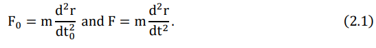
Here, t₀ and t represent the static and dynamic time intervals, respectively.

Differentiating the functional relationship between t₀ and t from equation (1.8) with respect to t₀ yields

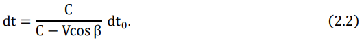
Substituting equation (2.2) into the expression for the dynamic force F in (2.1) yields

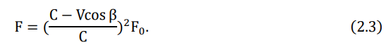
Equation (2.3) provides the functional relationship between the dynamic force F and the static force F₀. Equation (2.3) shows that when the speed of light, C, is finite and both the relative speed V and cosβ are nonzero, F differs from F₀. Furthermore, their difference increases with increasing speed V.

Application of the Functional Relationship Between Dynamic and Static Forces in Newtonian Mechanics

In this section, the functional relationship between dynamic and static forces, as given in equation (2.3), is employed to extend the scope of Newton’s second law and Newton’s law of universal gravitation in classical mechanics. The extended versions will be applicable to the calculation of not only forces between objects at relative rest but also to those between objects in relative motion. To distinguish these extended laws from their classical counterparts, we refer to them as the extended Newton’s second law of motion and the extended Newton’s law of universal gravitation, respectively.

Extended Newton’s Second Law of Motion

Newton’s second law describes the natural principle governing changes in an object’s state of motion under the influence of a force in a specific scenario, where the object exerting the force and the object experiencing it are at relative rest. Its mathematical expression is given by [2]

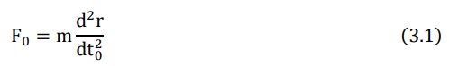
By using equations (2.2) and (2.3) to convert dt₀ and F₀ into dt and F, respectively, we obtain

This is the differential form of the extended Newton’s second law. The expression indicates that the mathematical form of the extended Newton’s second law is identical to that of the classical formulation. Consequently, it is speculated that the underlying physical interpretation of the extended law remains consistent with its classical counterpart. The extended Newton’s second law applies not only to the force calculations when the interacting bodies are at relative rest but also to those when they are in relative motion.

Extended Newton’s Law of Universal Gravitation

Similar to Newton’s second law of motion, Newton’s law of universal gravitation is believed to describe the gravitational force between two objects at relative rest [2]. Therefore, when the relative velocity between two objects is non zero, the gravitational force computed using Newton’s law of universal gravitation represents the static gravitational force, F₀, rather than the actual dynamic gravitational force between the two objects, F. That is,

Substituting the expression for F₀ from equation (2.3) into the above yields

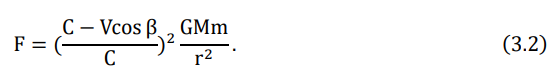
Equation (3.2) is the mathematical expression for the extended Newton’s law of universal gravitation. This extended law is applicable not only to the calculation of the gravitational force between objects at relative rest but also between objects in relative motion. Notably, when the relative velocity V between two interacting objects in motion is zero (V = 0), equation (3.2) reduces to the classical form of Newton’s law of universal gravitation. This clearly demonstrates that the extended law is compatible with the classical law, with the latter being a special case of the former when the relative velocity between two interacting objects in motion is zero.

Mathematical analysis of expression (3.2) reveals that if the extended Newton’s law of universal gravitation is used to compute the gravitational forces among celestial bodies, the orbital trajectories of the planets in the solar system would no longer be closed ellipses. Instead, the planets would follow nearly elliptical paths that do not close and continuously revolve around the Sun. Moreover, the orientation of these approximate ellipses would precess as the planets move, resulting in continual shifts in their perihelion. Therefore, the validity of the extended Newton’s law of universal gravitation can be verified by applying it to calculate planetary orbits and comparing the results with astronomical observations.

Application of the Functional Relationship Between Dynamic and Static Forces in Classical Electromagnetic Theory

In this section, the functional relationship between dynamic and static forces expressed by equation (2.3) is first employed to extend the applicability of Coulomb’s law in classical electromagnetism theory. The extended version of Coulomb’s law applies not only to calculating the electric field force between stationary point charges but also to that between point charges in relative motion. Subsequently, by applying the extended Coulomb’s law, a coherent theoretical derivation of several related laws in classical electromagnetism that were originally deduced from experimental observations by earlier researchers are provided. To distinguish the classical electromagnetic theory from its extended version, we refer to the latter as the extended classical electromagnetic theory.

Extended Coulomb’s Law for Point Charge Electric Fields

Coulomb’s law for electrostatic fields is a fundamental law of electromagnetism derived from experimental observations. It describes the natural variation of the electric field force between two point charges at relative rest [3]. In this case, the electric field force between the two point charges, a static force denoted by F₀, is given by

Substituting the expression for F₀ from equation (2.3) into the above yields

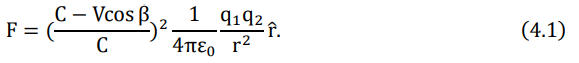
Equation (4.1) is the mathematical expression for the extended Coulomb’s law for point charge electric fields. Here, F represents the electric field force between the point charges q1 and q2, and V denotes the relative speed between the two point charges. Equation (4.1) shows that when the relative speed between the interacting point charges is zero (V = 0), the extended expression reduces to the classical Coulomb’s law for electrostatic fields. This confirms that the extended Coulomb’s law for point charge electric fields is consistent with Coulomb’s law for electrostatic fields, with the latter being a special case only applicable when there is no relative motion between point charges.

The extended Coulomb’s law for point charge electric fields is applicable not only to the calculation of static electric field forces between two point charges at rest but also to the computation of dynamic electric field forces between charges in relative motion. This extension significantly broadens the applicability of Coulomb’s law within classical electromagnetic theory.

Extended Coulomb’s Law for Line Charge Electric Fields

The distribution of positive and negative point charges in a conductor can be considered as positive and negative line charges. In the mathematical expression (4.1) for the extended Coulomb’s law for point charge electric fields, the velocity, V, represents the relative motion between two point charges. However, in a conductor, the motion of electrons is random and irregular, with both the magnitude and direction of their velocities being indeterminate random quantities. Currently, the macroscopic drift velocity of free electrons can only be indirectly determined by measuring the current [3]. Therefore, when applying expression (4.1) to calculate the electric field force between point charges in a line charge, we must multiply the macroscopic drift velocity V by a correction coefficient, that is,

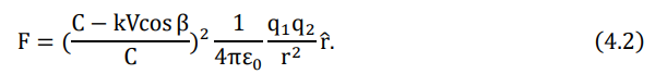
Equation (4.2) is the mathematical expression for the extended Coulomb’s law for line charge electric fields, incorporating an overall correction coefficient, k. In physics, the value of this coefficient is typically determined experimentally, similar to how constants such as G in the law of universal gravitation are established. Despite this, k for the macroscopic drift velocity in line charges can still be derived by analyzing the electromagnetic force between two current-carrying wires.

As shown in schematic diagram 2, consider two parallel current-carrying wires, L₁ and L₂, separated by a distance R. In wire L₁, the linear densities of both the positive and negative charges are λ1, whereas the macroscopic drift velocity of the negative charges is V_1. Additionally, the length of this wire is assumed to be infinitely long.

Alternatively, in wire L₂, the linear densities of both the positive and negative charge are λ₂, and the macroscopic drift velocity of the negative charges is V₂. The length of this wire, which is finite, is denoted by L₂. The currents in both wires flow in the same direction, and all the positive charges remain stationary.

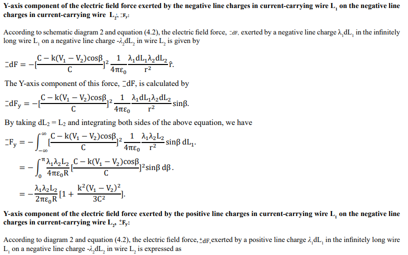
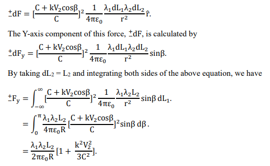
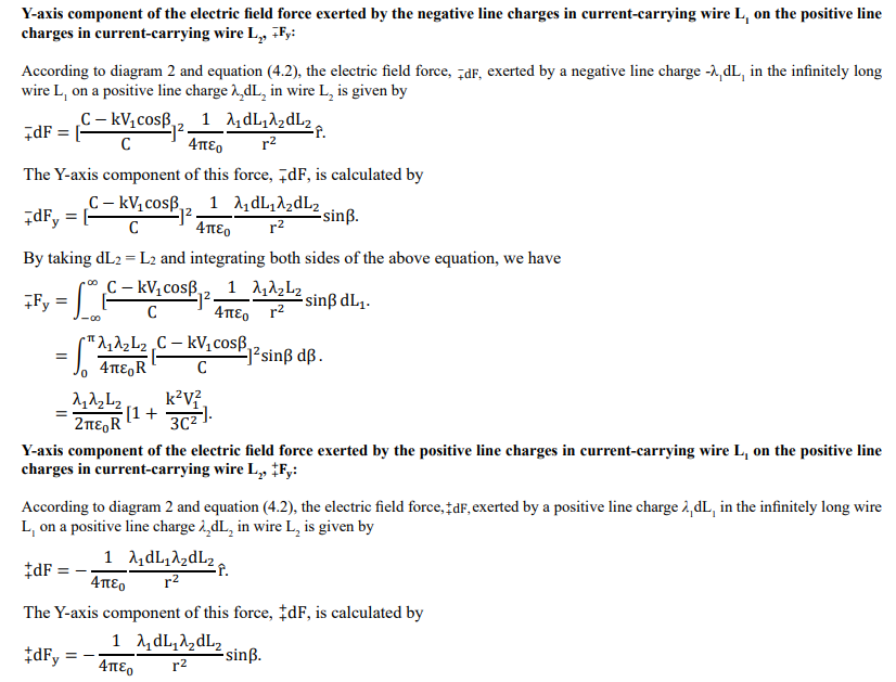
By taking dL₂ = L₂ and integrating both sides of the above equation, we have

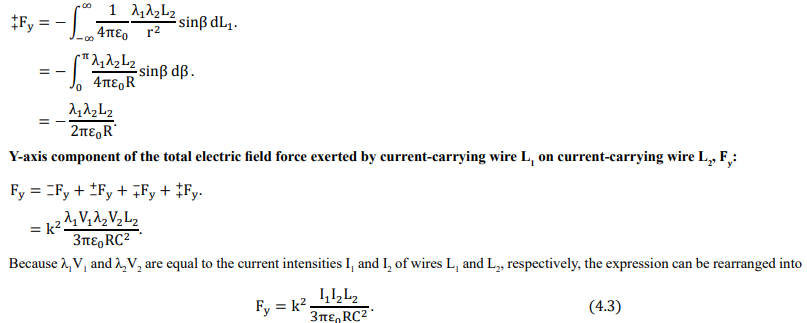
 Here, F_y denotes the Y-axis component of the total force exerted by the infinitely long wire L₁ on wire L₂, calculated using equation (4.2). Alternatively, according to classical electromagnetic theory, the Y-axis component of the force exerted by the infinitely long wire L₁ on wire L₂, F_y, is given by [3]

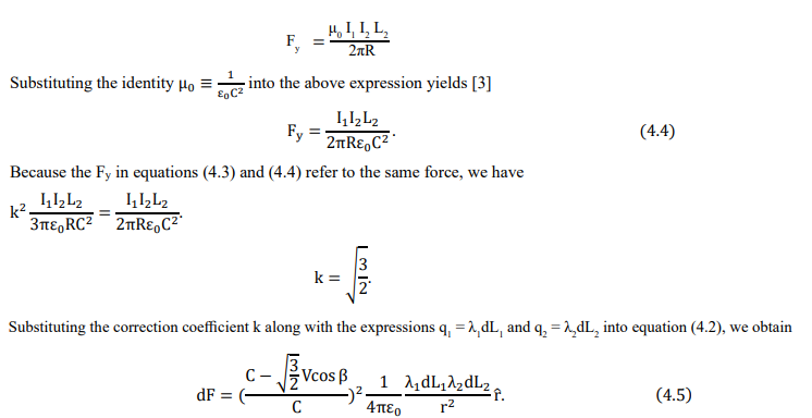
Equation (4.5) is the mathematical expression for the extended Coulomb’s law for line charge electric fields. Here, dF represents the electric field force between two different line charges λ₁dL₁ and λ₂dL₂, V denotes the macroscopic relative drift velocity between λ₁dL₁ and λ₂dL₂ and β refers to the angle between the line joining the two line charges and the macroscopic relative velocity V.

Application of the Extended Coulomb’s Law for Line Charge Electric Fields in Classical Electromagnetic Theory

In this section, the extended Coulomb’s law for line charge electric fields is employed to theoretically derive certain concepts and laws in classical electromagnetic theory. To distinguish the derived theorems from the conventional laws of classical electromagnetic theory, we prepend the term “extended” to the names of the derived laws and designate them as theorems.

Extended Ampère Theorem

Next, the extended Coulomb’s law for line charge electric fields is used to theoretically calculate the electric field force between two current elements. The resultant mathematical expression is termed the extended Ampère theorem.

As depicted in schematic diagram 3, we assume the distance between two current elements dL1 and dL2 is r, and the angle between the line joining them and the positive X-axis is β. In current element dL1, the negative charges move at an angle, θ, relative to the positive X-axis. Meanwhile, current element dL₂ is located at the origin, the negative charges of which move along the X-axis.

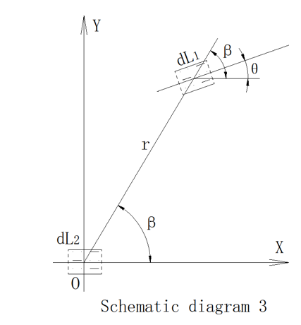
We assume that in current element dL₁, the macroscopic drift velocity of the negative charges is V₁, whereas the positive charges remain stationary. Additionally, the linear densities of both the positive and negative charges are λ₁. Alternatively, in current element dL₂, the macroscopic drift velocity of the negative charges is V₂, whereas that of the positive charges remain at zero. The linear densities of both types of charges are λ₂. According to the mathematical expression (4.5) for the extended Coulomb’s law for line charge electric fields, the electric field force, dF, owing to the interaction between the line charge elements λ₁dL₁ in dL₁ and λ₂dL₂ in dL₂ is expressed as

 

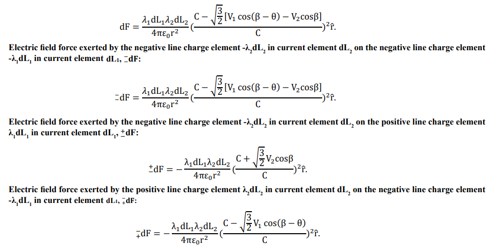
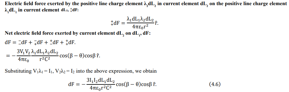
Equation (4.6) is the mathematical expression of the extended Ampère theorem describing the force between two current elements. While this expression differs from the traditional mathematical form of Ampère’s law, in the special case where the two current elements are parallel and one of them is infinitely long, the result obtained from the extended Ampère theorem coincides exactly with that derived from Ampère’s law [3].

Extended Biot–Savart Theorem

In this section, based on the physical definition of magnetic induction B and using the mathematical expression of the extended Ampère theorem, equation (4.6), the mathematical expression of the extended Biot–Savart theorem is derived.

According to the definition of magnetic induction B, when in equation (4.6) we set dL₁ = 1m, I₁ = 1A, and θ = 0°, the magnetic field intensity produced by the current element I₂dL₂ at a distance r, denoted by dF, is given by [3]

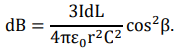
The above expression is the extended Biot–Savart theorem. Although it differs from the traditional mathematical form of the Biot–Savart Law, in the limit of an infinitely long current element, the results obtained from the extended Biot–Savart theorem are identical to those of the conventional Biot–Savart law [3].

Extended Faraday’s Theorem of Electromagnetic Induction

Faraday’s law of electromagnetic induction is a classic law of electromagnetism derived from experimental observations. It describes the natural phenomenon in which a changing magnetic field induces an electromotive force in a conductor. The sources of the varying magnetic field can be broadly classified into those generated by permanent magnets and those induced by current-carrying conductors [3]. Notably, the magnetic field generated by a magnet results from the motion of electrons around atomic nuclei, which exhibit both high numbers and complex trajectories. Thus, calculations based on the extended Coulomb’s law for line charge electric fields are not yet applicable. Therefore, the following sections focus exclusively on electromagnetic induction phenomena resulting from the magnetic fields of current-carrying conductors.

The mathematical expression for Faraday’s law of electromagnetic induction is given by [3]

According to the definition of magnetic flux, when the magnetic field lines are perpendicular to the plane formed by the closed loop, the expression for Faraday’s law of electromagnetic induction can be expressed as [3]

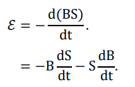
In the above equation, the first term on the right-hand side of the equation represents the motional electromotive force as described in classical electromagnetic theory, and the second term corresponds to the induced electromotive force. Next, using the extended Coulomb’s law for line charge electric fields, the variation patterns for both the motional and induced electromotive forces are calculated. The resultant mathematical expressions are referred to as the extended motional electromagnetic induction theorem and the extended induced electromagnetic induction theorem, respectively.

Extended Motional Electromagnetic Induction Theorem

As depicted in schematic diagram 4, consider an infinitely long current-carrying conductor L with a current I, where free electrons move along the positive X-axis at speed V1. A closed loop, abcd, is formed by a conductor, where segment ab is free to move and travels along the negative Y-axis at a speed of V. The distance R denotes the separation between the charges in segment ab and current-carrying conductor L.

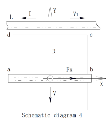
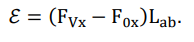
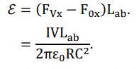
According to the physical definition of electromotive force, the motional electromotive force ε generated at the two ends of segment ab due to its motion is equal to the difference between the electric field force FVX along the X-axis experienced by a unit negative charge in the moving state and the electric field force F_0X along the X-axis experienced by the same negative charge in the stationary state in segment ab, multiplied by the length of segment ab, L_ab, that is [2,3],

By applying the mathematical expression of the extended Coulomb’s law for line charge electric fields, i.e., equation (4.5), the expressions for F_VX and F_0X are given by

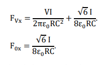
Based on this, the mathematical expression for the motional electromotive force ε across the two ends of segment ab is expressed as

Because the direction of the induced current in segment ab is the same as that in the infinitely long conductor L, the magnetic fields generated by the two cancel each other within the area enclosed by the closed loop. Consequently, a negative sign is introduced to the induced electromotive force ε. The mathematical expression for the extended motional electromagnetic induction theorem is therefore given by [3]

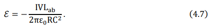
Because BdS = d∅ [3], the above expression can be rearranged into

The above equation is the mathematical expression of Faraday’s law of electromagnetic induction [3]. This result indicates that the extended Coulomb’s law for line charge electric fields can be used to derive Faraday’s law of electromagnetic induction, which was originally deduced from experimental observations. Consequently, equation (4.7), which represents the mathematical formulation of the extended motional electromagnetic induction theorem in terms of electric fields, is equivalent to Faraday’s law of electromagnetic induction, which is expressed in terms of magnetic fields. This observation also indirectly verifies the correctness of the extended Coulomb’s law for line charge electric fields.

Extended Induced Electromagnetic Induction Theorem

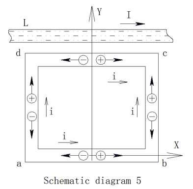
As shown in schematic diagram 5, consider a current-carrying conductor L with a current I, and assume abcd is a closed loop formed by a conductor. When the current in conductor L flows along the positive X-axis, the mathematical expression (4.5) of the extended Coulomb’s law for line charge electric fields is applicable to compute the forces on both the positive and negative charges in the closed loop. The resultant force directions on these charges are as indicated in diagram 5.

Schematic diagram 5 shows that an induced electromotive force ε exists between points a and c in the closed loop abcd. Under the influence of this induced electromotive force ε, the negative charges (free electrons) in the loop split into two streams flowing from point c to point a, thereby generating an induced current i in the loop. As negative charges accumulate at point a, a static electric field is established between points a and c, the magnitude of which is equal to that of ε but opposite in direction. At this point, because the forces exerted by the induced electromotive force and the static electric field on the charges in the loop are equal in magnitude and opposite in direction, the charges in the loop become macroscopically stationary, and the induced current in the loop vanishes (i = 0). If the current I in conductor L remains constant, the positive and negative charges in the closed loop will remain macroscopically at rest, and the induced current will continue to be zero.

Alternatively, when the current in L increases, according to the mathematical expression (4.5) of the extended Coulomb’s law for line charge electric fields, the electric field generated by L will exert a greater force on the charges in the closed loop, such that the electric field force due to L becomes greater than the static electric field force formed by the charges within the loop. In this case, an induced current will continue to arise in the closed loop flowing toward point c, thereby increasing the static electric field strength until the forces on the charges once again reach equilibrium and the induced current vanishes.

Conversely, when the current in L decreases, based on to the mathematical expression (4.5) of the extended Coulomb’s law for line charge electric fields, the force exerted on the charges in the closed loop by the electric field produced by L diminishes accordingly, making it smaller than the static electric field force generated by the charges in the loop. At this point, an induced current (denoted as current i in the diagram) flows toward point a that is opposite in direction to the original induced current. This current reduces the static electric field strength in the loop until the forces on the charges reach equilibrium once more and the induced current again vanishes.

The above describes the principle underlying the generation of the induced electromotive force and induced current. Nevertheless, formulating a complete mathematical expression for induced electromagnetic induction solely within the theoretical framework of the extended Coulomb’s law for line charge electric fields remains a significant challenge that requires further in-depth investigation.

Conclusion

By incorporating the finite speed of light into classical physics, this paper successfully expands the scope of application of classical physics. And validation of the extended theory through experimentally derived laws of classical electromagnetism confirmed that this new theory correctly reflects the objective laws of the interaction between objects in nature. Through a summary of the theoretical derivation results in this paper, the main conclusions can be drawn as follows:

a. The finite speed of light induces variations in the relative time between objects in relative motion. These temporal variations, in turn, alter the interaction forces between the objects.

b. The changes in gravitational force caused by the variations in the relative motion speeds between celestial bodies are the fundamental cause of planets orbiting along elliptical paths and exhibiting precession.

c. The generation of magnetic fields is intrinsically linked to the finite propagation speed of light. If the speed of light were infinite, the magnetic fields around a current-carrying conductor would vanish, the magnetic needle in Oersted’s experiment would not deflect, and magnetic materials would not exist in nature. Therefore, the finite speed of light is a necessary condition for the presence of magnetic fields.

d. Magnetic fields, which arise from the relative motion between positive and negative charges. The N-pole and S-pole of a magnet originate from the relative motion between electrons and atomic nuclei within the magnet, they are generated simultaneously and are indivisible. Therefore, magnets cannot exist in the form of monopoles.

e. By applying the new theory of classical physics presented in this paper, multiple experimentally established laws of classical electromagnetism can be derived, thereby contributing to the consolidation and streamlining of the overall framework of classical electromagnetic theory.

References

1. Newton, I. (1833). Philosophiae naturalis principia mathematica (Vol. 1). G. Brookman.
2. Kittel, C., Knight, W. D., Ruderman, M. A., Purcell, E. M., Aguilar Peris, J., & Pujal Carrera, M. (1965). Berkeley physics course.
3. Purcell, E. M. (1963). Berkeley physics course. Electricity and magnetism.
4. Weinberg, S. (1995). The quantum theory of fields (Vol. 2). Cambridge university press.