A Computational Algorithm For The Hardy Function Z(t), Utilizing Sub-Se-quences of Generalized Cubic Gauss Sums, With An Overall Operational Complexity O((t⁄εt)[0.25, 0.3]{log(t)}2+o(1)) FOR ∈[1023−35]

Introduction

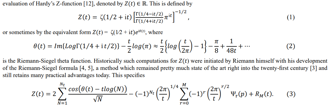
Interest in novel methodologies for the computation of the Riemann zeta function ζ(S ) along the critical line S = 1 \ 2 + it remains strong, given its fundamental importance to the distribution of the primes. Practically, computations along the critical line come down to the

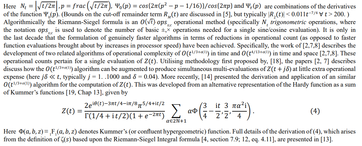
The algorithms developed by [2,7] rely primarily on the observation (made by D. R. Heath-Brown [see 7] on analysis presented in [24, section 5.2]) that subsections, or ‘blocks’, of terms that constitute the main part of the Riemann-Siegel formula could be re-written in the form of a series of quadratic Gaussian sums, albeit with very specific parameters. The algorithm of rests on an analogous observation but applied to asymptotic approximations for the terms of (4). A general quadratic Gaussian sum of length N is defined by

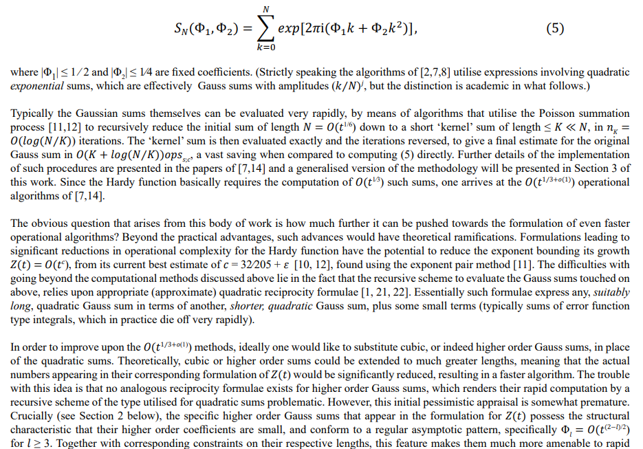
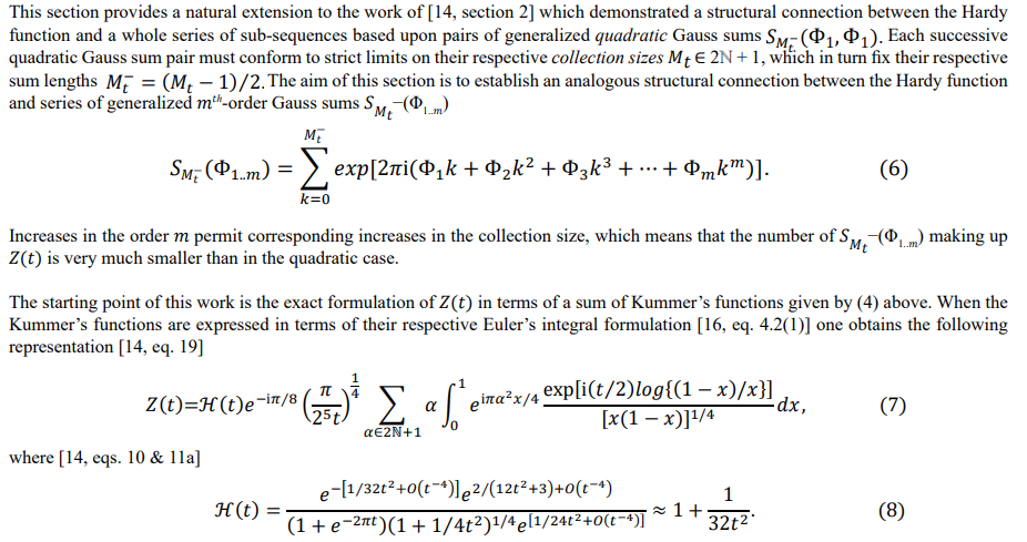
Formulating Hardys z-Function into Generalized mth-order Gauss Sums

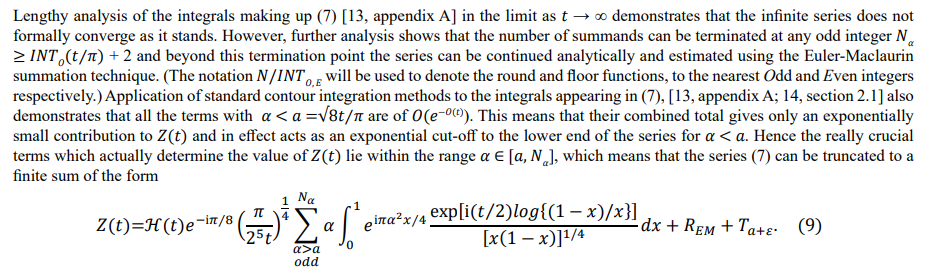
Combining Together Collections of Integrals That Form the Main Sum (9) for z(t)

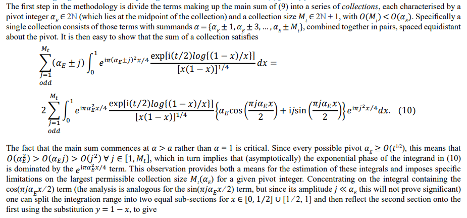
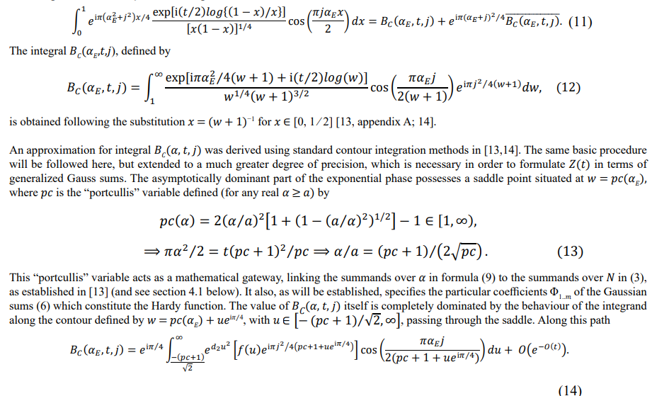
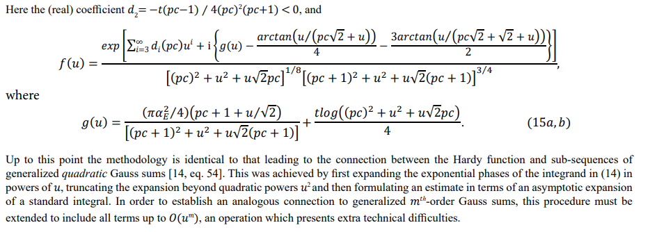Extended analysis of integral B_c(a_E¸t j) 

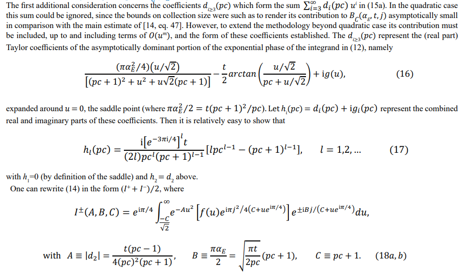
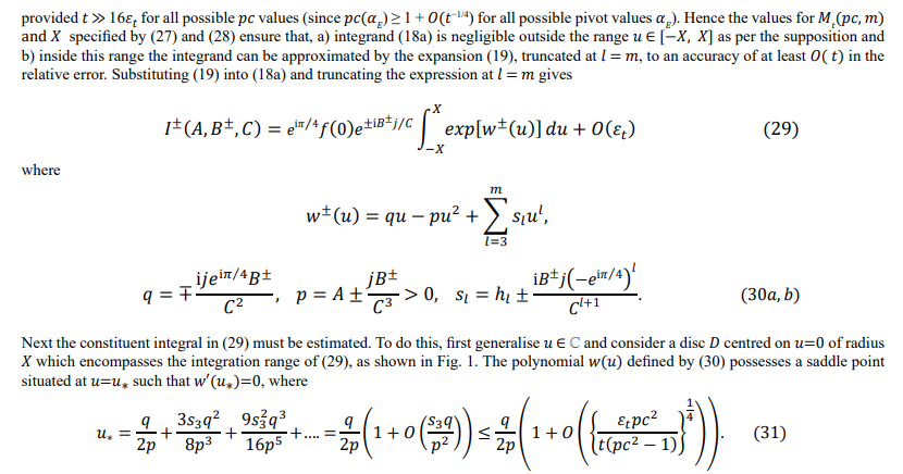
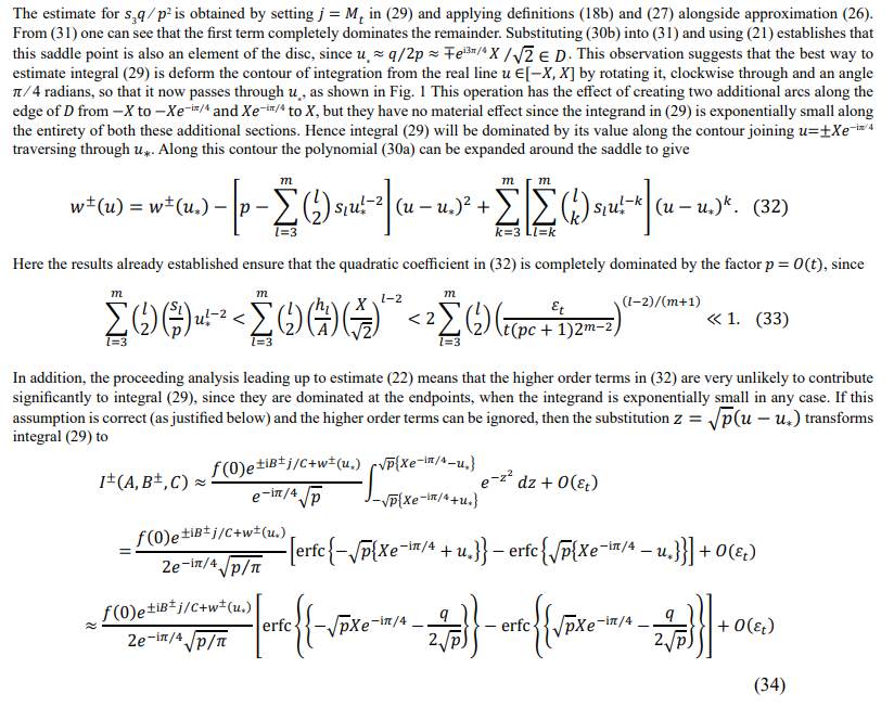
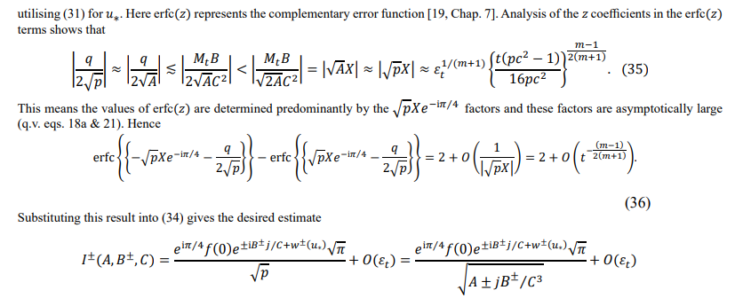
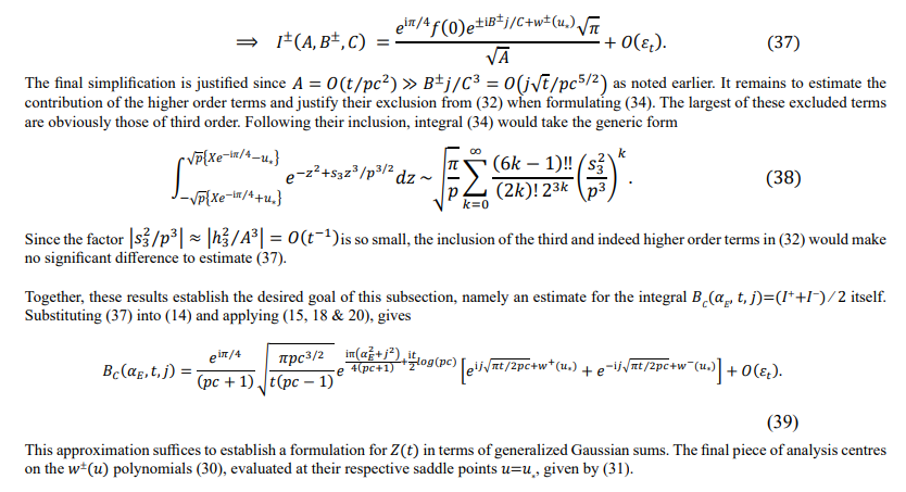
The polynomial expressions W^±(µ^∗).

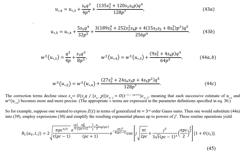
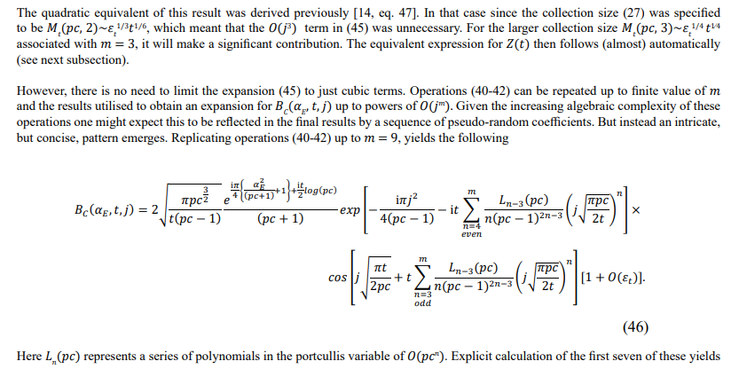
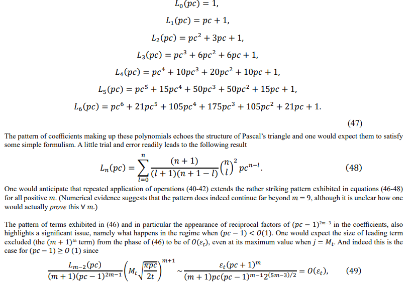
z^(t) composed in terms of Generalized m^th-order Gauss Sums

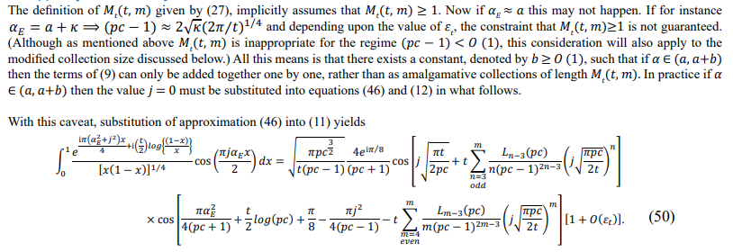
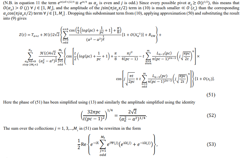
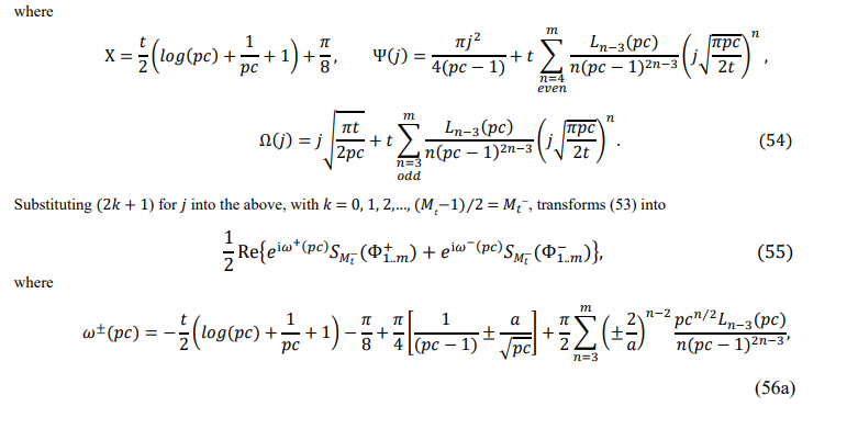
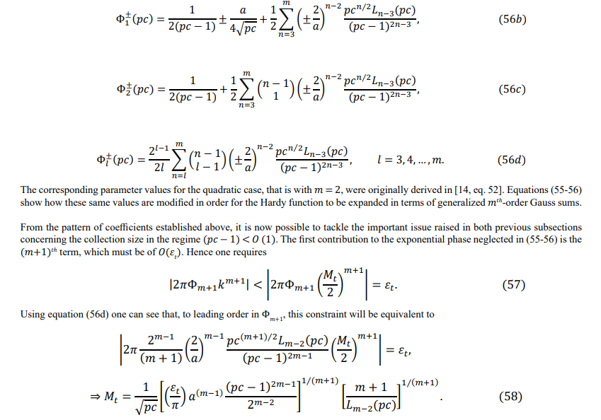
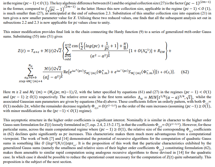
Efficient computation of the particular Generalized Gauss Sums constituting z(t)

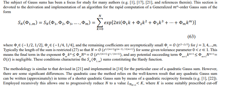
Derivation of the reciprocity formula for generalized m^th-order Gauss sums

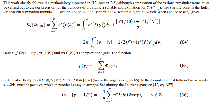
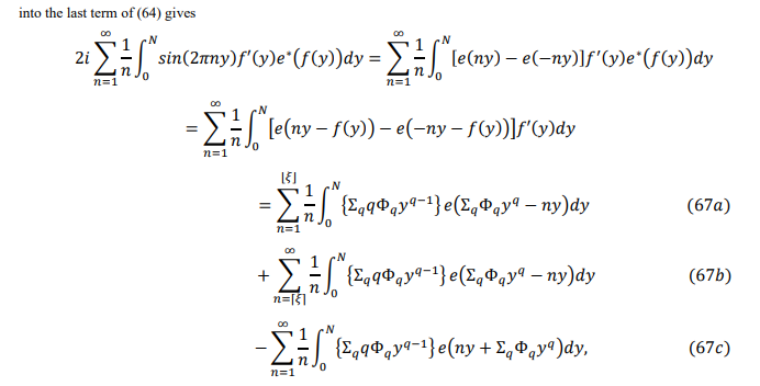
Estimation of Term (67a)

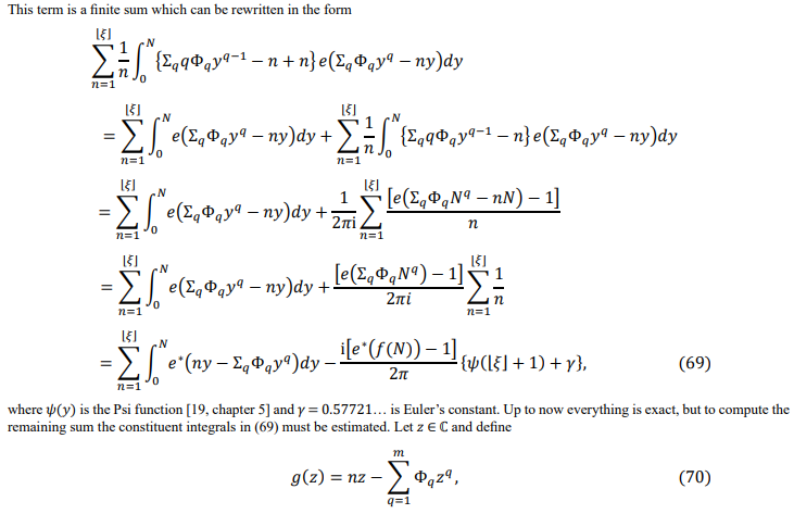
Estimation of Terms (67b) and (67c)

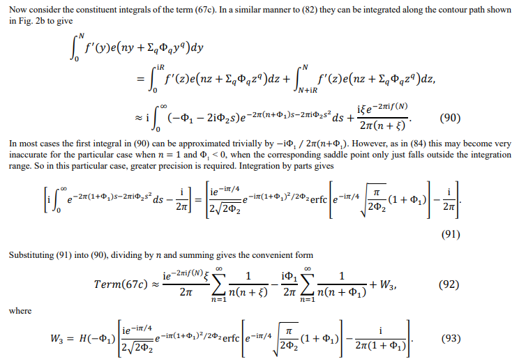
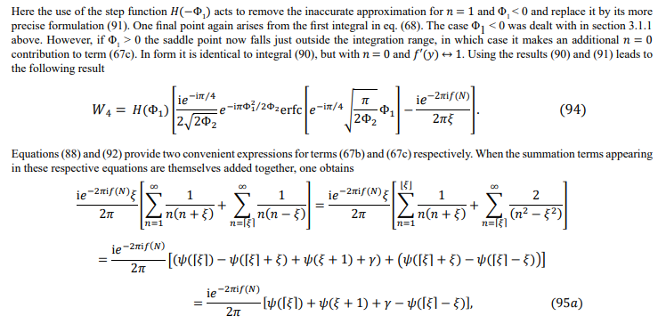
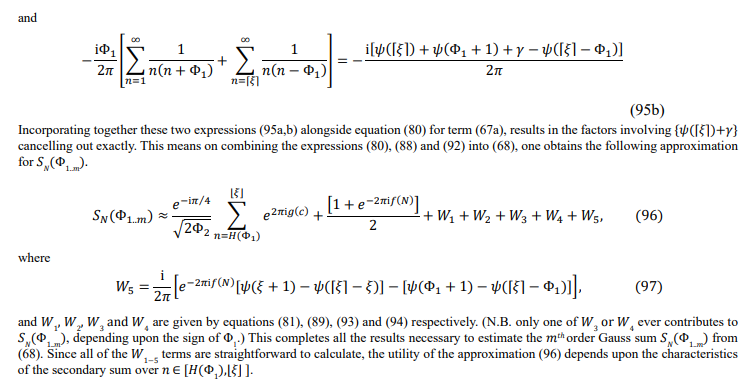
Analysis of the secondary sum in (96)

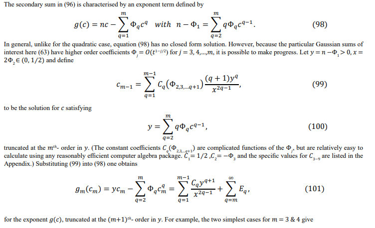
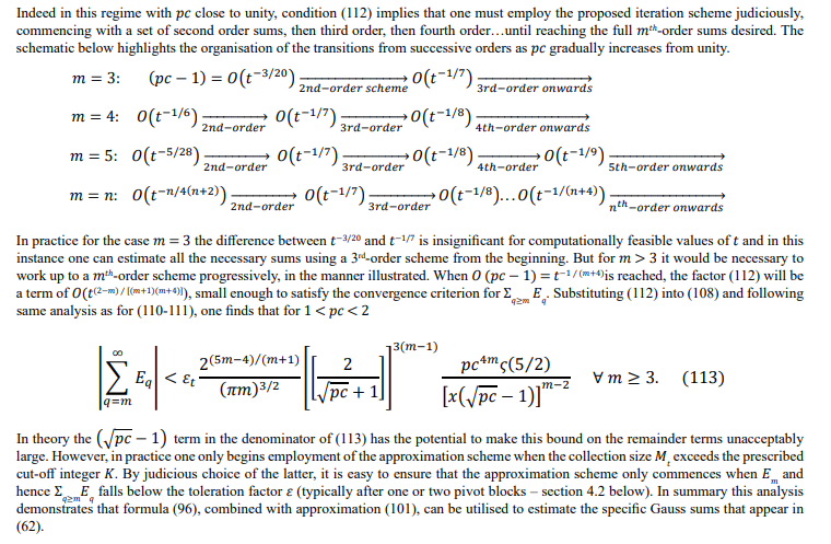
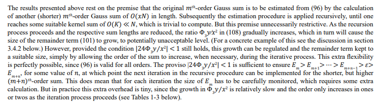
A recursive scheme for the efficient computation of a Generalized m^th-order Gaussian sumS_N (Φ ), satisfying coefficient  conditions (63).

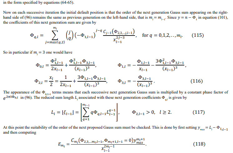
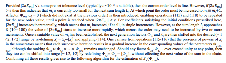
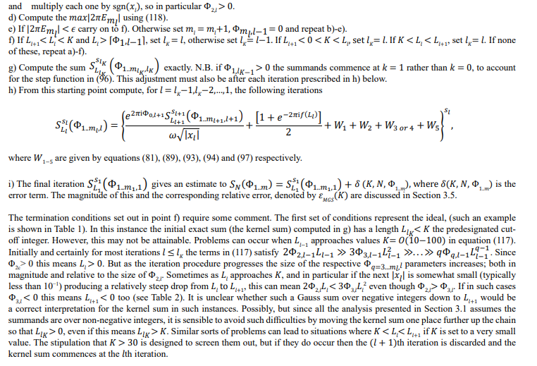
An algorithm for the recursive computation of a Generalized m^th-order Gauss Sum S_N(Φ_1,m ), with N« 1, m≥3 and coefficients  Φ_1..m satisfying the specific conditions set out in equation (63). (algorithm MGS)

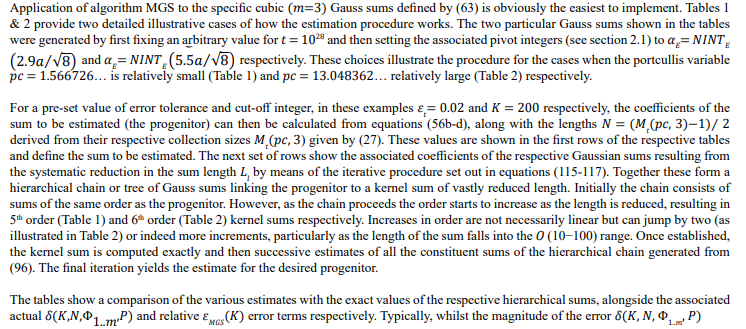
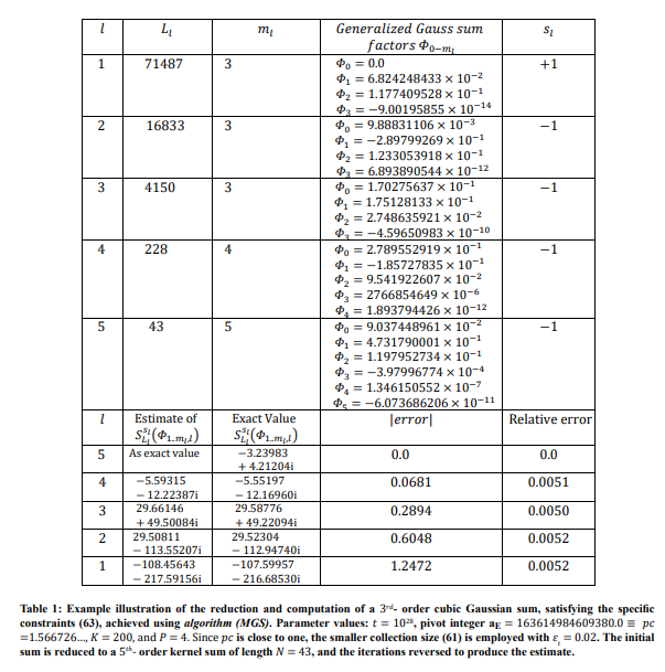
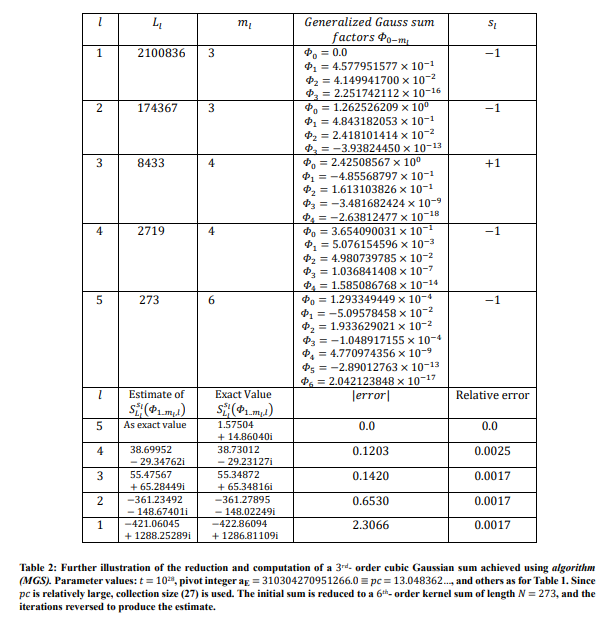
Sample computations using algorithm MGS

Cubic Gauss sums (m= 3)

Quartic Gauss Sums (m = 4): the reductive bound on cut-off k.

Error Analysis

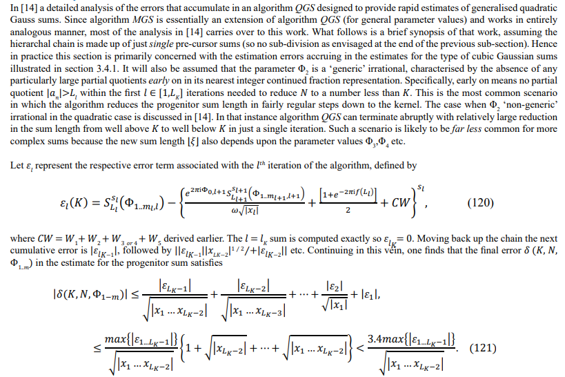
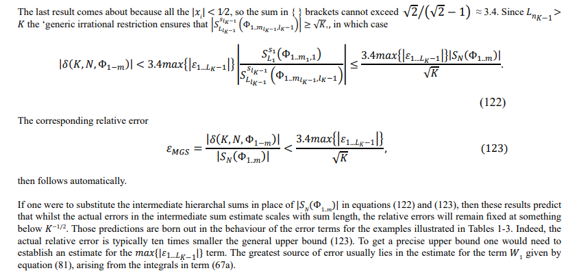
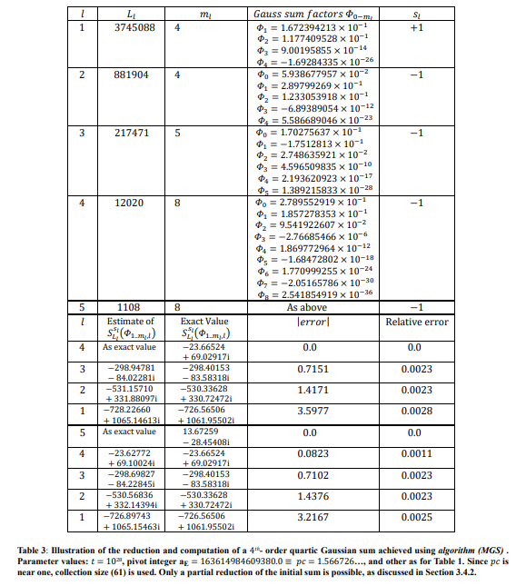
Since these get more complicated with the order of the sum, the €1...L_K−1|} is usually associated with the error in the first iteration €1...L_K−1 beyond the kernel sum. In the tables one can see the relative error jumping up in the first couple of iterations, before stabilising thereafter. In the quadratic case discussed in [14] it was possible to put a specific bound on this term. For the higher order sums discussed here it much more difficult to formulate such a bound. Rather than pursue this, one can take the pragmatic view that more precise estimates can be simply computed by including more terms in the approximations developed in section 3.1.1. As ever, greater precision imposes a higher operational count, and one must balance the demands for high computational speed against high accuracy.

In conclusion, the results presented in this section demonstrate that the specific type of Generalized Gaussian sums which constitute the Hardy function in (62) can be computed very efficiently by means of algorithm MGS. Large scale calculations of the Hardy function itself, utilising this methodology, are presented in the next section.

Sample Computations of z(t) for large t utilising Cubic Gauss Sums

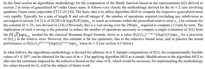
Formulation of a hybrid summation formula for the estimation of z(t)

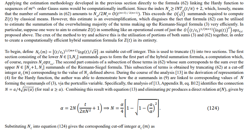
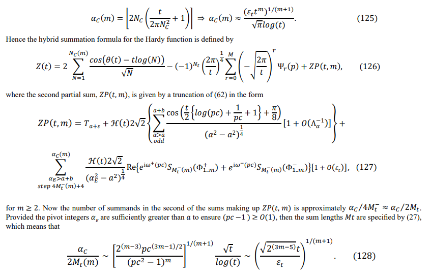
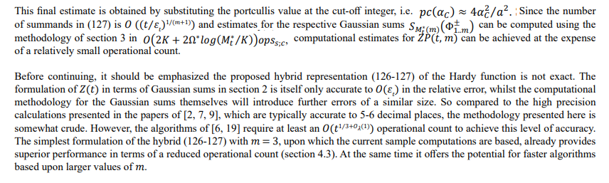
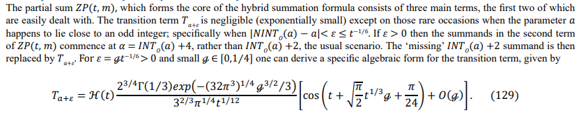
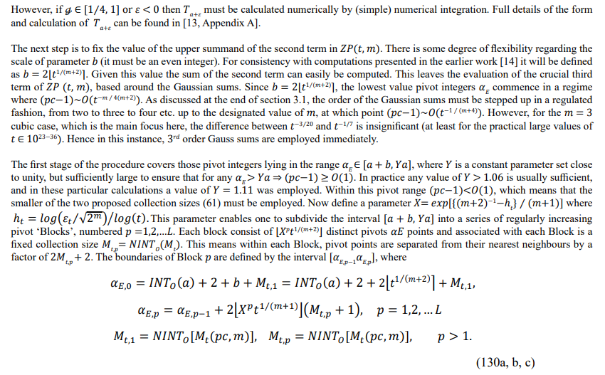
Computational scheme for the hybrid summation formula

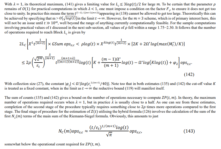
Sample Computations

Thanks to the invaluable web-based database [9] of sample calculations of the Hardy function, it is possible to compare the performance

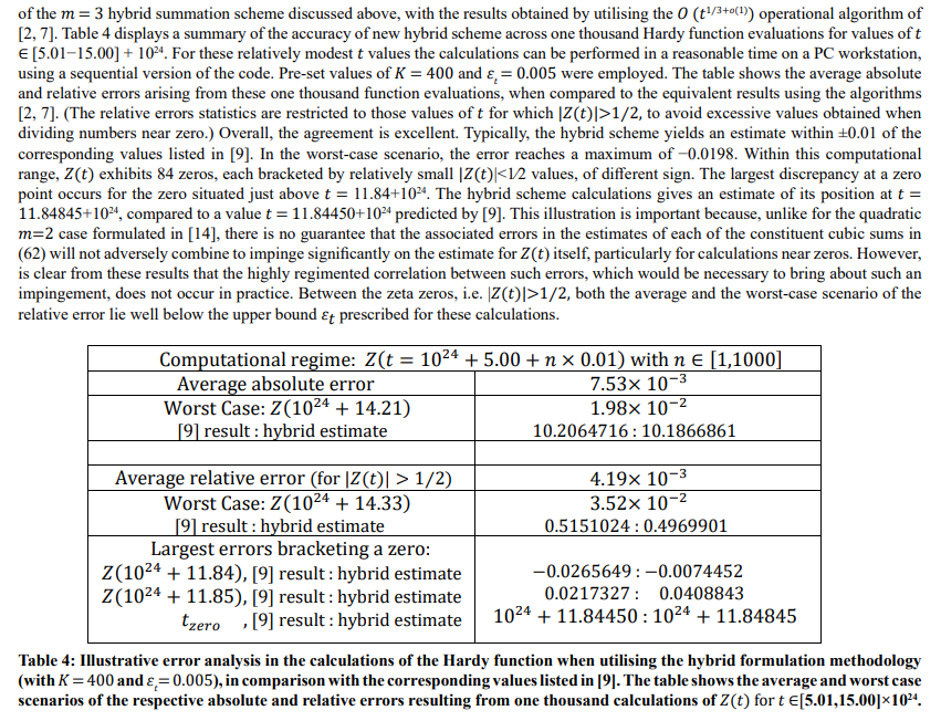
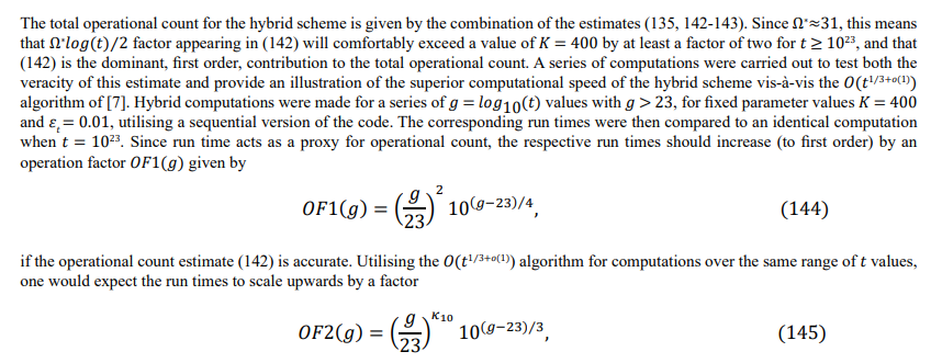
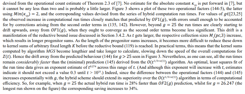
Table 5 shows a similar comparison of the accuracy of the new hybrid scheme for a selection of t values where z(t) exhibits an unusually large local maximum/minimum, compared to other such points in its vicinity. (Since z(t) is unbounded, much greater values of |z(t)| certainly exist, although for larger, computationally unfeasible t values.) Details of the methodology utilised to identify narrow intervals along the critical line where such points are likely (but not guaranteed) to occur, are discussed in [9]. The latter reference also provides details of many examples where |z(t)|>10³, whilst [23] highlights some calculations of especially large values of |z(t)|>10⁴, utilising the z(t(1)) algorithm. The large |z(t)| computations shown in Table 5 are for t> 10²⁸, covering the highest possible range of computationally feasible t values.

For these particular computations, a parallelised version of the hybrid summation code was developed for implementation on the ARCHER2 UK National Supercomputing Service (http://www.archer2.ac.uk) hosted by the University of Edinburgh. Open-source variants of this hybrid code are now freely available from the repository [15], along with documentation describing its implementation and some sample output files. ARCHER2 is a HPE Cray EX supercomputing system with a total of 5860 nodes, each consisting of two 2.25GHz, 64 core AMD EPYC7742 processors with access to 256GB of memory (https://www.archer2.ac.uk/user-guide/hardware/). Most of the computations listed in Table 5 were run using 4-8 nodes and required between 3-12 hours of CPU time. However, the highest calculations, when t ≥ 1032, were carried out during one of the periodic ARCHER2 Capability Days sessions, which give users the opportunity to run large scale jobs, at no budgetary cost, using many nodes. The t ≥ 10³² calculations highlighted in the Table 5 employed 512-1024 nodes and typically required between 1-3 hours of CPU time.

Looking at the results shown in Table 5, one can see the agreement between the hybrid estimates and the corresponding values published in [9, 23] is excellent, with all the relative errors lying far below the prescribed value of €_t = 0.005. The absolute errors are also very low, which is noteworthy since such errors tend to reach a maximum in and around points where |z(t)| is large. Of course, if more accurate estimates are desired, then one can simply reduce the user prescribed value of €_t , at the expense of a marginal increase in run times. One of the chief difficulties encountered for computations where t > 10²⁸ is the potential for catastrophic round-off error, resulting from the fact that Fortran double precision variables can only represent numbers to an accuracy of some thirty-three significant figures. In order to circumvent this issue, the main Fortran codes in the repository [15] utilise certain C subroutines from the PariGP computer library [20], accurate to many thousands of digits, for those particular calculations where round-off error is problematic. Indeed, it is anticipated that the repository code should be capable of carrying out computations for t~10⁴⁰ or even a little beyond, before the need for quadruple precision reals becomes imperative. However, although feasible, calculations on this scale would exhaust the supercomputer budgetary resource allocation very generously awarded in support of this work.

Table 5: Illustrative calculations of the Hardy function for t > 10²⁸ utilising the hybrid formulation methodology, compared to the corresponding values listed in [9, 23]. At these particular t values the modulus of z(t) is unusually large. For all the hybrid computations, the precision setting was∈_t = 0.005 with k ∈ [598, 992].

Conclusions

Acknowledgments

The authors would like to acknowledge the help and advice of the ARCHER2 UK National Supercomputing Service User Support Team in facilitating the computational results presented in this paper. In particular, the help of Dr Mario Antonioletti (EPCC, The University of Edinburgh) is acknowledged. Establishment of the GitHub computational repository [15] was funded under the EPSRC/ARCHER2-eCSE grant scheme (grant no. 11-7).

References

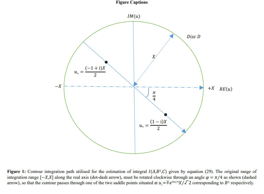
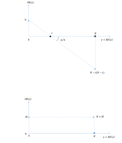
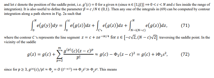
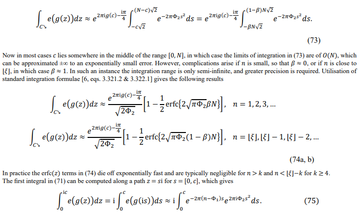
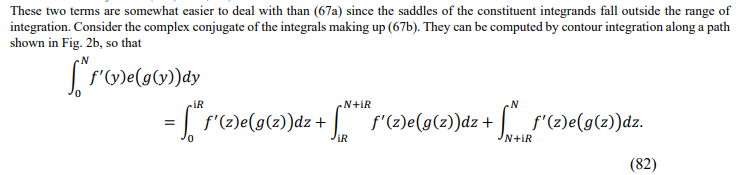
Figures 2a and 2b: Contour integration paths utilised to estimate integrals given by equations (71: Fig. 2a) and (82: Fig. 2b). In each case the path of integration along the real line (solid arrow) is substituted by the complex contour path traced out by the dashed arrows. Estimates for the constituent line segments forming the respective contour paths are derived in the text.

References

- Berndt, B. C. & Evans, R. J. 1981 The Determination of Gauss Sums. Bull. Amer. Math. Soc. 5(5), 107-129.
- Bober, J. W. & Hiary. G. A. 2018 New computations of the Riemann zeta function on the critical line. Experimental Mathematics 27(2), 125-127.
- Borwein, J. M., Bradley, D. M. & Crandell, R. E. 2000 Computational strategies for the Riemann zeta function. J. Comp. Appl.Math. 121, 247-296.
- Edwards, H. M. 1974 Riemann’s zeta function, New York, Dover Publications.
- Gabcke, W. 1979 Neue Herleitung und Explizite Restabschätzung der Riemann-Siegel-Formel. Ph.D. thesis, Göttingen.
- Gradshteyn, I. S. & Ryzhik, I. M. 2007 Table of Integrals, Series and Products. (7th edition) Jeffrey, A. & Zwillinger, D. (eds.) Elsevier Academic Press.
- Hiary G. A. 2011 Fast methods to compute the Riemann zeta function. Annals of Mathematics 174, 891-946.
- Hiary G. A. 2011 A nearly-optimal method to compute the truncated theta function, its derivatives and integrals. Annals of Mathematics 174, 859-889.
- Hiary G. A. 2017 Fast methods to compute the Riemann zeta function.
- Huxley M. N. 2005 Exponential sums and the Riemann zeta function V. Proc. Lond. Math. Soc. 90, 1-41.
- Iviac A. 2003 The Riemann Zeta-Function. Dover Publications, Inc., New York (republication of work published in 1985 by John Wiley & Sons, New York).
- Iviac A. 2013 The Theory of Hardy’s Z-Function. Cambridge Tracts in Mathematics, Cambridge University Press.
- Lewis, D. M. 2015 The development of a hybrid asymptotic expansion for the Hardy function z(t), consisting
main terms, some 17% less than the celebrated Riemann-Siegel formula.
- Lewis, D. M. 2017 A computational algorithm for the Hardy function z(t)utilising sub-sequences of generalised quadratic Gauss sums, with an overall complexity operational complexity 0(t\t),1\3 {log(t)2+0(1))
- Lewis, D. M. 2025 Hardy Code-Detailed Documentation, GitHub repository.
- Luke, Y. L. 1969 The special functions and their approximations (Vol. 1), New York & London, Academic Press.
- Montgomery, H. L. & Vaughan R. C. 2006 Multiplicative Number Theory: I. Classical Theory. (Ch.9) Primitive characters and Gauss sums pp 282-325, Cambridge Studies of Advanced Mathematics 97, Cambridge University Press.
- Odlyzko, A. M. & Schönhage A. 1988 Fast algorithms for multiple evaluations of the Riemann zeta function. Trans. Amer. Math. Soc. 309, 797-809.
- Olver, F. W. J., Lozier, D. W., Boisvert, R. F. & Clark, C. W. 2010 NIST Handbook of Mathematical Functions, Cambridge University Press.
- Pari/GP computer algebra library 2003-2026 (Originally developed by Cohen, H. et. al. at the University of Bordeaux).
- Paris, R. B. 2008 An Asymptotic Expansion for the Generalised Quadratic Gauss Sum. Applied Mathematical Sciences 2(12), 577-592.
- Siegel, C. L. 1960 Uber das quadratische Reziprozitätsgesetz Zahlkörpern Nachr. Akad. Wiss. Göttingen Math.-Phys. Kl. No. 1, 1-16.
- Tihanyi, N. 2019 Numerical computing of extremely large values of the Riemann-Siegel Z-function. PhD thesis, Doctoral School of Informatics, Numeric and Symbolic Computations, Eötvös Lorand and University.
- Titchmarsh, E. C. 1986 The theory of the Riemann zeta-function, 2nd edn. Oxford, Clarendon Press.