
Environmental Science and Climate Research(ESCR)
ISSN: 2996-2498 | DOI: 10.33140/ESCR


Research Article - (2025) Volume 3, Issue 1
Smoke in your Eyes: Investigating the Effects of Wind Power on Weather Trends and Climate using Time Series Analysis
Received Date: Mar 10, 2025 / Accepted Date: Apr 08, 2025 / Published Date: Apr 15, 2025
Copyright: ©Â©2025 Dr. Keith Johnson. This is an open-access article distributed under the terms of the Creative Commons Attribution License, which permits unrestricted use, distribution, and reproduction in any medium, provided the original author and source are credited.
Citation: Johnson, K. (2025). Smoke in your Eyes: Investigating the Effects of Wind Power on Weather Trends and Climate using Time Series Analysis. Env Sci Climate Res, 3(1), 01-12.
Abstract
Time series analysis developed in the previous report for UK mean summer temperature has been applied to further examples of weather trends, including temperature, rainfall and Sahara dust, and so at global, regional, national and local levels, in an attempt to assess whether wind power is having a deleterious effect on weather patterns. The analysis involves detrending weather data by calculating first differences and then computing the cross-correlation function, or CCF with wind power capacity. The calculations are benchmarked using atmospheric CO2 concentration. The consistency of a significant correlation is tested by detrending using linear residuals and then calculating the CCF on the basis of the residuals, corrected for autocorrelation using the Cochrane-Orcutt procedure [1-4]. In four cases, where the data were reliable, the analysis provided a clear distinction in favour of wind power as a putative cause of the weather trends, in preference to atmospheric CO2 concentration. Where the quality of the data was less reliable, the outcome was inconclusive. Nevertheless, it would seem that our efforts to mitigate anthropogenic global warning with wind power might well be having a deleterious effect on weather patterns.
Keywords
Climate Change, Wind Power, Time Series Analysis, Weather Trends, Berkeley GMST, Sahara Dust Cross-Correlation, CCF Autocorrelation Cochrane-Orcutt
Introduction
The current consensus among climate scientists that the science behind climate change is settled and accounted for by anthropogenic global warming due to rising CO2 levels in the atmosphere has led to each and every adverse weather event being ascribed to such climate change. Yet could there not be other causes which have a deleterious effect on weather patterns, at least in addition to anthropogenic global warming, even if not as the main cause of climate change? This article is an attempt to address this question using time series analysis, especially in regard to the effects of wind power.
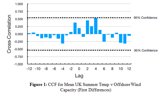
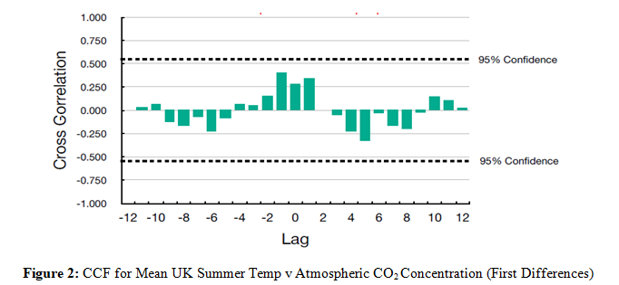
Recently, this technique was applied to UK Mean Summer temperatures from the UK Met Office [1]. First, the statistical significance of the data was determined by comparing with the mean and standard deviation of the whole time series and using the Wald Wolfowitz Runs Test. On this basis, only the rising trend in the last decade or so (> 2009) was possibly significant. The trend was then compared with various potential causes: atmospheric CO2, global carbon emissions, China carbon emissions etc. By detrending, using first differences, and computing the cross- correlation function, or CCF, only offshore wind generating capacity gave a significant level of cross-correlation in the CCF Compared with the results for atmospheric CO2.
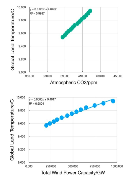
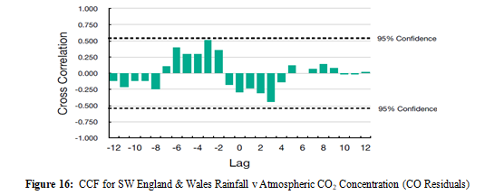
The cross-correlation persisted, and indeed was amplified, when a different method of detrending was used and autocorrelation taken into account using the Cochrane Orcutt procedure. Of course, correlation is not causation. However, lack of correlation certainly excludes causation. Hence, if the rising trend is significant, it is not caused by atmospheric CO2 levels whereas the hypothesis that it is associated with offshore wind generating capacity cannot be rejected. At first glance, it may seem improbable that offshore wind power could affect the weather. However, as discussed in the previous paper [1], Bodini et al [17] already noted that ‘… Long-term meteorological measurements in the vicinity of wind plants can also be affected by wind plant wakes… aggregated wakes from multiple turbines, i.e., wind plant wakes, can extend more than 50 km downwind of a wind plant, offshore in stable conditions…’. Moreover, an analysis of wind turbine wake dynamics carried out there on the basis of Bernouilli’s principle showed that extracting large amounts of energy from wind turbines must lead to low pressure down wind of the turbines. With prevailing westerly winds and largely offshore wind farms, this meant the creation of a low pressure region in the North Sea. By sucking hot air from Africa, this low pressure region might then provide a mechanism for the increase in the mean UK summer temperature and also account for the Cerberus heat wave in 2023 and Sahara dust plaguing Europe in recent years. Data analysis was performed using Numbers spreadsheets, one for each data set, on an Apple iPad pro. The spreadsheet developed for the previous study of UK mean summer temperatures served as a template. A typical table of contents is shown below: Table of Contents Sheet 1 Total Wind Power Capacity and Berkeley Global Mean Surface Temperature Sheet 2 Linear regression, Durbin Watson statistic, Cochrane Orcutt corrections Sheet 3-1 CCF 1st Differences Berkeley Global Mean Surface Temperature v Total Wind Power Capacity Sheet 3-2 CCF Linear Residuals Berkeley Global Mean Surface Temperature v Total Wind Power Capacity Sheet 3-3 Ditto - after Cochrane Orcutt Correction for Autocorrelation ρ = 0.70926 Sheet 3-4 Ditto - Cochrane Orcutt Correction for Autocorrelation ρ = 0.735 Sheet 3-5 CCF 1st Differences Berkeley Global Mean Surface Temperature v Atmospheric CO2 Concentration Sheet 4 Workings Σ(xt − with xt, yt the first differences in the parameters at time, t and et′ = et − ρ . et−1 where ρ is the lag-1 autocorrelation in the x-series and et′ , the corrected residual at time t. In sheet 3.5, the CCF based on first differences for the benchmark, atmospheric CO2, is shown. Sheet 4 contains various bits and bobs used in preparing the data for analysis. More details can be found in the previous report [1]. The data for global surface land temperature were taken from BerkeleyEarth.com and total wind power capacity corresponds to figure 17.14 of Brugger, taken from references [2,6,7] respectively. The temperature data were presented as an anomaly from the 1850- 1900 average and were corrected accordingly. The data for Vienna air temperature and wind power capacity in Austria correspond to figures 17.6 and 17.7 from Brugger taken from references [2,8,9]. Similarly, the Paderborn data are based on figures 17.12 and 17.13 from Brunner, and derive from references [10,11]. The original rainfall deficit was converted to a cumulative deficit. As the data did not cover the entire time range under investigation, 2009-2023, linear extrapolation was used to fill the gaps. Note the wind power data is simply the number of wind farms in the Paderborn district, not their capacity. For the example SW England and Wales Rainfall v UK Wind power capacity, the rainfall data are taken from Dee and derived from from data taken from the UK Met Office [12]. The wind power capacity was taken over from the previous report but are also based on UK Met office data. The benchmark data for atmospheric CO2 are also taken over from the previous report [1]. The spreadsheet contains extra sheets 2.1, 3.5.1-3.5.3, which allow the Cochrane-Orcutt procedure to be applied to the linear residuals for atmospheric CO2 For the Sahara dust example, as commented on by Varga, there are very few direct measurements of Saharan dust deposit in Europe. Instead, the data used is derived from modelling, which ‘… represent the only useable quantitive data sources of daily dust deposition in the area…’. The data from Varga was converted to cumulative dust deposition [13-16]. The data were obtained by digitising the published figures using the web digitiser, https:automeris.io/wpd else entered manually. The spreadsheets are available on the iCloud on request to the author and a pdf version can be found as Supplementary information on Zenodo: https://doi.org/10.5281/zenodo.1426706. 1.Global Land Surface Temperature Figure 4 (top) shows the strong correlation between the global land surface temperature and atmospheric CO2: Figure 4: Global Land Temperature v Atmospheric CO2 (top) and Global Land Temperature v Total Wind Power Capacity (bottom) However, very good correlation is also found between the global land surface and total wind power capacity, figure 4 (bottom). Yet detrending, using first differences, yields no significant correlation in the CCF for atmospheric CO2: As in the case of UK mean summer temperatures, this is amplified when linear residuals are used for detrending and the Cochrane-Orcutt procedure applied: Thus time series analysis quite clearly differentiates between total wind power capacity and atmospheric CO2 as putative causes for the rise in global land temperature. This would imply that the temperature goes up as the CO2 goes down and leads the CO2 concentration. So it seems fair to dismiss atmospheric CO2 concentration as a cause for the increase in local air temperature. Thus the outcome is inconclusive in regard to distinguishing between wind farms and atmospheric CO2 as putative causes. However, it seems to exclude the latter. Moreover, the data for wind farms are incomplete and based on the number of wind farms rather than their generating capacity. So it is not surprising the former also fails. Perhaps the question should be readdressed, if more accurate data becomes available. (iv) Rainfall in South West England and Wales Indeed the CCFs based on first differences and linear residuals also show positive correlation in both cases, although at negative lag for atmospheric CO2. See sheets 3.5.1-3.5.3 of spread sheet WT Power v Rainfall in the Supplementary Information for details. However, the residuals are strongly autocorrelated. In these circumstances, as stressed by Beaulieu et al, it is important to include a correction for autocorrelation in order to avoid false positives [16]. Consequently, the Cochrane-Orcutt procedure was also applied to the linear residuals from atmospheric CO2 as well as those from UK Wind Capacity. After application of the Cochrane- Orcutt procedure, significant correlation remains in the CCF for Rainfall versus UK Wind Capacity:and persists in the CCF for rainfall versus atmospheric CO2 concentration yet at negative lag: Thus it seems more probable that the increase in rainfall on the time scale under investigation is due to the increase in wind power capacity rather than to changes in atmospheric CO2 concentration. (v) Sahara Dust Yet there are few direct measurements of dust deposition in Europe and, like Varga, we have to rely model simulations as the only source of quantitative data. The modelled cumulative dust correlates strongly with both atmospheric CO2 and total wind capacity: Figure 17: Cumulative Sahara Dust v Atmospheric CO2 Concentration (top) and Cumulative Sahara Dust v Total Wind Power Capacity So again the outcome is inconclusive in regard to distinguishing between total wind power capacity and atmospheric CO2. As noted by Varga, while the modelled dust data are in good qualitative agreement with experimental values, where they exist, the modelled deposition rates quantitatively underestimate the experimental ones. Perhaps this accounts for the failure of the former [13,14]. Time series analysis developed in the previous report for UK mean summer temperature has been applied to further examples of weather trends, including temperature, rainfall and Sahara dust, at global, regional, national and local levels [1]. In four cases, where the data were reliable, the analysis provided a clear distinction in favour of wind power as a putative cause of the weather trends, in preference to atmospheric CO2 concentration. Where the quality of the data was less reliable, the outcome was inconclusive. Nevertheless, the results seem to suggest that our efforts to mitigate anthropogenic global warning with wind power might well be having a deleterious effect on weather patterns. 1. Johnson, K. (2024). Blowing in the Wind: A Time Series Analysis of Mean UK Summer Temperature.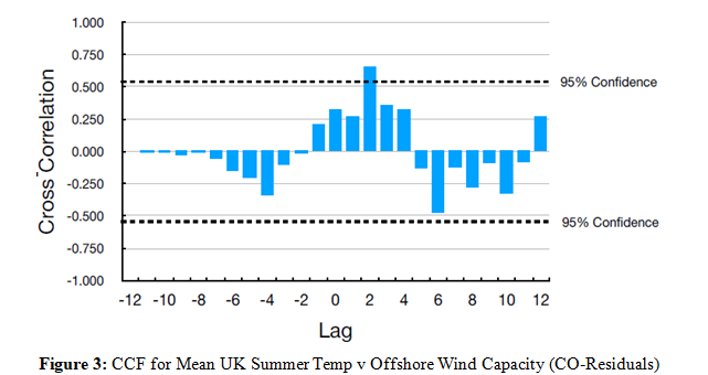
Meanwhile, further evidence for the contention that wind power may be affecting the weather has been published by Brugger in his book, ‘Windwahn: Der Windwahn und seine klimatischen Konsequenzen’ [2]. Wind mania in English. Here the author suggested there was qualitative correlation between (i) Global land surface temperature and total wind power capacity; (ii) Vienna air temperature and local wind power capacity; and (iii) Rainfall deficit and wind farms in and around Paderborn, Germany. Below, the time series analysis developed for the UK mean summer temperatures is applied to these examples, along with (iv) Rainfall in SW England and Wales v. UK offshore wind capacity and (v) Sahara dust against total wind power capacity on the same time scale 2009-2023. The latter was proposed as a test in the original report [1]. The results are benchmarked against atmospheric levels of CO2 over the same period.Data Analysis and Methods
In sheet 1, various correlations between the parameters for examples (i)-(v), eg. Global surface temperature and total wind power capacity, and for the benchmark atmospheric CO2, are calculated along with linear regressions. In sheet 2, linear residuals are determined from the regression equations of sheet 1, the Durbin Watson statistic calculated, and estimates of the extent of serial correlation, ρ determined, and then applied in the Cochrane-Orcutt procedure [3,4]. In sheet 3.1, the cross-correlation function, CCF, based on first difference is calculated from the formula:x ) . (yt−l − y )/[Σ(xt − x )2]1/2 . [Σ(yt − y )2]1/2 ,
, y, the mean values of these quantities, with lag, l, using a tabular method for spread sheets [5]. The 95% confidence limits are then given by ±1.96√N with N the number of values. As a check on the validity of the method, the cross-correlation at lag, l = 0, calculated in sheet 2, using the in-built function, CORREL, is compared with the value determined via the tabular method. Sheet 3.2 shows the CCF based on the linear residuals determined in sheet 2 and the results of the validity test. Sheets 3.3 and 3.4 repeat the calculations using residuals corrected via the Cochrane-Orcutt procedure for different values of ρ, from sheet 2, using the formula:Results


(ii) Vienna Air Temperature
As noted by Brugger, the increase in Vienna air temperature tends to match that in Austrian wind power capacity:
Again, the positive correlation is amplified when the CCF is calculated from the linear residuals and the Cochrane-Orcutt procedure applied: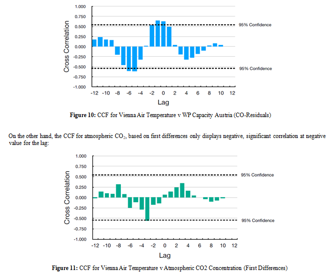
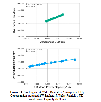
(iii) Rainfall Deficit in Paderborn District, Germany
Of course, changes in weather patterns and climate affect not just temperature but also other meteorological variables, such as rainfall. As an example Brugger cites data from the Paderborn district in Germany. Indeed, there appears to be a strong correlation between cumulative rainfall deficit and the number of wind farms in the Paderborn area of Germany: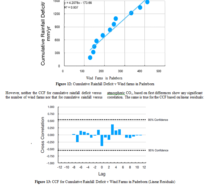
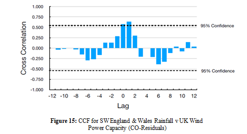
The rainfall data reported by Dee [12] for South West England and Wales constitute a 12-month running average, which shows strong correlation with both atmospheric CO2 and UK Wind Capacity:
As discussed in Varga et al [13,14], the number and intensity of Saharan dust storm events identified in Europe have been increasing over the last decade, due to the role of ongoing climate change. Increased warming of the Arctic has led to decreasing temperature contrast between higher and lower latitudes which drives the jet stream. Because of deviations in the west-east pattern, low pressure atmospheric systems which blow through the Atlas mountains, causing severe dust storms, have turned northwards and reached central and northern Europe. On the other hand, it was posited in the previous report that increases in Sahara dust might be linked to increasing offshore wind capacity in the North Sea. As indicated there, an acid test to distinguish between these scenarios would be to apply the current time series analysis to cumulative dust data.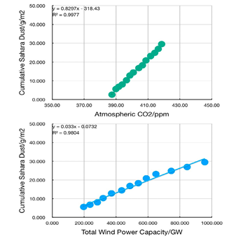
(bottom)
However, neither the CCF for cumulative dust versus total wind power capacity nor that for cumulative dust versus atmospheric CO2, based on first differences, show any significant correlation.
The same is true for the CCF for total wind power capacity based on linear residuals after application of the Cochrane-Orcutt procedure with ρ = 0.70926: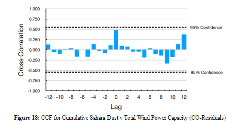
Conclusion
Acknowledgements
The author is grateful for useful discussions with Antonio Pierfederici.References
2. Brugger, M. (2023). Windwahn: Der Windwahn und seine kli- matischen Konsequenzen. novum premium Verlag.
3. “Durbin–Watson Statistic.” In Wikipedia, Octo- ber 9, 2023. https://en.wikipedia.org/w/index.php?ti- t l e = Du r b i n % E 2 % 8 0 % 9 3 Wa t so n _ st a t i st i c & ol - did=1179357537.
4. “Cochrane–Orcutt Estimation.” In Wikipedia, December 18, 2023. https:// en.wikipedia.org/w/index.php?title=Co-chrane%E2%80%93Orcutt_estimation&oldid=1190613841.
5. El-Hajj, A., Kabalan, K. Y., & Khoury, S. (2004). The use of spreadsheets to calculate the convolution sum of two fi- nite sequences. International Journal of Engineering Educa- tion, 20(5), 867-871.
6. Rohde, R. (2021). Global temperature report for 2021. Berk- ley Earth.
7. WWEA Half Yearly Report 2022. World Wind Energy Associ- ation, n.d. https:// wwindea.org/wp-content/uploads/2022/11/ WWEA_HYR2022.pdf.
8. Interessen Gemeinschaft Windkraft Österreich. “Windfakten-.” Accessed November 14, 2024. https://windfakten.at/?xml- val_ID_KEY%5B0%5D=1234.
9. Hiebl J., Orlik A. “Wiener KlimaRückblick 2021.” ccca.ac.at, 2022. https://ccca.ac.at/fileadmin/00_DokumenteHaupt- menue/02_Klimawissen/Klimastatusbericht/KSB_2021/ Kli- marueckblick_Wien_2021.pdf.
10. Bernemann M. “Anpassungsstrategien in der Trinkwasserver- sorgung“. Energie Wasserpraxis, 2019. https://www.dvgw. de/medien/dvgw/wasser/klimawandel/ anpassungsstrate- gien-wasserversorgung-energie-wasser-praxis-maerz-2019. pdf.
11. Wagenknecht A. “Rotmilan und Windenergie im Kreis Pad- erborn: Untersuchung von Bestandsentwicklung und Bruter- folg“. FA Wind, 2019. https://www.fachagenturwindenergie. de/fileadmin/files/Veroeffentlichungen/
12. FA_Wind_Analyse_Rotmilan_Paderborn_08-2019.pd- f#page21.
13. John Dee’s Climate Normal: “Rainfall in South West England and Wales (Part 2).” Substack.com, January 11, 2024. https:// open.substack.com/pub/jdeeclimate/p/rainfall-in-south- west-england-and?r=1omo87&utm_medium=ios.
14. Varga, G., Rostási, Á., Meiramova, A., Dagsson-Waldhau- serová, P., & Gresina, F. (2023). Increasing frequency and changing nature of Saharan dust storm events in the Carpath- ian Basin (2019–2023)–the new normal?. Hungarian Geo- graphical Bulletin, 72(4), 319-337.
15. Varga, G. (2020). Changing nature of Saharan dust deposition in the Carpathian Basin (Central Europe): 40 years of iden- tified North African dust events (1979–2018). Environment international, 139, 105712.
16. Pérez, C., Nickovic, S., Baldasano, J. M., Sicard, M., Roca- denbosch, F., & Cachorro, V. E. (2006). A long Saharan dust event over the western Mediterranean: Lidar, Sun photometer observations, and regional dust modeling. Journal of Geo- physical Research: Atmospheres, 111(D15).
17. Beaulieu, C., Gallagher, C., Killick, R., Lund, R., & Shi, X. (2024). A recent surge in global warming is not detectable yet. Communications Earth & Environment, 5(1), 576.